
In the age of data-driven decision making, having the ability to combine and analyze data from multiple sources is crucial. One powerful tool that can assist in this process is Google Sheets. Whether you are a business owner looking to analyze sales data or a marketing professional wanting to merge data from various campaigns, Google Sheets offers a user-friendly interface and powerful features.
In this article, we will explore different methods for combining data in Google Sheets. We’ll cover everything from basic data import and appending data from multiple sheets to leveraging functions like VLOOKUP and QUERY to merge data from different sources. By the end of this article, you’ll have the knowledge you need to efficiently combine and analyze data in Google Sheets, empowering you to make informed decisions based on comprehensive insights.
Inside This Article
- Understanding Data Combination in Google Sheets
- Methods for Combining Data in Google Sheets
- Using the CONCATENATE function
- Using the JOIN function
- Using the QUERY function
- Using the Importrange function
- Conclusion
- FAQs
Understanding Data Combination in Google Sheets
Data combination is a crucial process when working with large sets of data in Google Sheets. It allows you to merge and consolidate different data sources, making it easier to analyze and draw insights. Whether it’s combining data from multiple sheets, using formulas to merge data, or simply concatenating text, Google Sheets provides various methods to accomplish this task.
By combining data from different sheets, you can bring together related information and create a comprehensive view. To import data from another sheet, use the IMPORTRANGE function. This function allows you to specify the source sheet and range, enabling you to pull data from a different tab or workbook. By importing multiple ranges, you can merge data from multiple sheets into one.
The QUERY function is another powerful tool for combining data in Google Sheets. It allows you to perform SQL-like queries on your data, fetching specific columns or rows based on your criteria. Using the SELECT, WHERE, and JOIN clauses within the QUERY function, you can merge data from multiple sheets, filter for specific conditions, and join tables based on matching values.
If you have data in separate sheets that share a common key, you can use the VLOOKUP function to combine them. VLOOKUP searches for a value in the first column of a range and returns a corresponding value from another column. By applying this function across multiple sheets, you can merge data based on a common identifier, such as customer or product ID.
The CONCATENATE function is particularly useful when you want to merge text or combine values from different cells. It allows you to join text strings or cell references together, creating a merged result. This can be handy when combining first names and last names, joining addresses, creating unique identifiers, or combining any other text-based data.
With these methods at your disposal, you can effectively combine and merge data in Google Sheets. Whether you’re working with multiple sheets, using formulas to merge data, or concatenating text, Google Sheets offers a versatile set of tools to simplify the data combination process. By utilizing these functions, you can streamline your workflow and gain deeper insights from your data.
Methods for Combining Data in Google Sheets
When working with Google Sheets, there may come a time when you need to combine data from different sheets or merge information from different columns. Thankfully, Google Sheets offers several methods to help you accomplish this task efficiently. In this article, we will explore three effective methods for combining data in Google Sheets.
1. Importing Data from Different Sheets
If you have multiple sheets with relevant data, you can easily import and combine them into one sheet using the IMPORTRANGE function. This powerful function allows you to pull data from another sheet or even another Google Sheet file.
To use this method, start by opening the sheet where you want to import the data. In an empty cell, enter the formula “=IMPORTRANGE(“Sheet URL”, “SheetName!Range”)”. Replace “Sheet URL” with the URL of the source sheet and “SheetName!Range” with the specific range of cells you want to import.
Once you have entered the formula, press Enter, and Google Sheets will prompt you to give permission to access the source sheet. After granting permission, the data from the specified range in the source sheet will be imported into your current sheet.
2. Using the QUERY Function
The QUERY function is a versatile tool in Google Sheets that allows you to extract and manipulate data based on specific criteria. It is especially useful when combining data from different sheets with different structures.
To use the QUERY function, select an empty cell where you want the combined data to appear. Enter the formula “=QUERY({Sheet1!A:Z; Sheet2!A:Z}, “SELECT * WHERE Col1 <> ””)”. Replace “Sheet1” and “Sheet2” with the names of your source sheets, and “A:Z” with the range of columns you want to include.
The QUERY function combines the data from the specified sheets and filters out any rows with empty values in the first column. You can adjust the query to include specific columns or apply additional conditions based on your requirements.
3. Using the CONCATENATE Function to Merge Data
If you need to merge data from different columns within the same sheet, the CONCATENATE function can come in handy. This function allows you to combine text values or cell references and join them into one cell.
To merge data using CONCATENATE, select an empty cell where you want the merged data to appear. Enter the formula “=CONCATENATE(Cell1, Cell2, Cell3, …)” and replace “Cell1”, “Cell2”, “Cell3”, and so on with the specific cells or cell references you want to combine.
The CONCATENATE function will combine the values from the selected cells into one merged cell. You can also add additional text or separators within the formula using quotation marks.
By using these methods, you can efficiently combine data in Google Sheets, whether it’s from different sheets or within the same sheet. Experiment with these techniques and explore the possibilities of data manipulation in Google Sheets to streamline your workflow and improve your data analysis.
Using the CONCATENATE function
One useful function in Google Sheets for combining data is the CONCATENATE function. This function allows you to merge text or cell values from different cells into a single cell.
To use the CONCATENATE function, you need to specify the text or cell references you want to combine. For example, if you have two cells containing the first name and last name of a person, you can use CONCATENATE to merge them into a full name in a separate cell.
Here’s an example to illustrate how to use the CONCATENATE function. Suppose you have cell A2 with the first name “John” and cell B2 with the last name “Doe”. In cell C2, you can enter the formula “=CONCATENATE(A2, ” “, B2)” to combine the contents of cells A2 and B2 with a space in between. The result will be the full name “John Doe” in cell C2.
The CONCATENATE function can also be used to merge more than two cells. For example, if you have cells A2, B2, C2, and D2 containing the first name, middle name, last name, and suffix of a person, respectively, you can use a formula like “=CONCATENATE(A2, ” “, B2, ” “, C2, “, “, D2)” to combine all the components into a single cell. The result will be the full name with the suffix, if applicable.
Additionally, you can combine text and cell references in the CONCATENATE function. For instance, you can merge a text string with the value in a particular cell. To do this, simply include the text inside quotation marks. For example, the formula “=CONCATENATE(“Hello, “, A2)” will combine the text “Hello, ” with the value in cell A2.
The CONCATENATE function can be especially useful when you need to create customized strings or concatenate values from different cells in Google Sheets. It provides a simple and efficient way to merge data and create dynamic content in your spreadsheets.
Remember, if you want to use the CONCATENATE function with multiple cells or values, separate them with commas inside the function. And always enclose text strings in quotation marks.
Using the JOIN function
Another powerful way to combine data in Google Sheets is by using the JOIN function. The JOIN function allows you to merge text from different cells into a single cell, separated by a specified delimiter.
To use the JOIN function, you simply need to provide the delimiter and the range of cells you want to combine. Here’s an example:
=JOIN(", ", A2:A5)
This will combine the values from cells A2 to A5, separated by a comma and a space. You can change the delimiter to any character or string of characters you prefer.
One useful application of the JOIN function is when you have a list of values in separate cells and you want to create a comma-separated list. For example, if you have a list of names in column A, you can use the JOIN function to create a single cell with all the names, separated by commas.
By combining the JOIN function with other functions like FILTER or SORT, you can even create dynamic and customized combinations of data in Google Sheets.
The JOIN function is a versatile tool that can be used in various scenarios, such as merging multiple columns into one, combining values from different cells, or creating a formatted list. It provides flexibility and convenience when working with data in Google Sheets.
Using the QUERY function
One powerful feature in Google Sheets is the QUERY function. This function allows you to extract specific data from a range of cells based on certain criteria or conditions. It is especially useful when combining data from multiple sheets into a single sheet.
To use the QUERY function, start by specifying the range of cells you want to pull data from. This could be a single sheet or multiple sheets. Next, define the query itself by using a SQL-like syntax. You can filter the data, sort it, and even perform calculations.
For example, let’s say you have two sheets: “Sales” and “Expenses”. You want to combine the data from both sheets and only show the total sales amount from a specific region. You can use the QUERY function to achieve this.
The formula would look like this:
=QUERY({Sales!A1:C, Expenses!A1:C}, "SELECT SUM(Col3) WHERE Col2 = 'Region A' LABEL SUM(Col3) 'Total Sales'")
In this example, we’re pulling data from columns A to C in both the “Sales” and “Expenses” sheets. We’re then selecting the sum of the third column (total sales) where the second column (region) matches ‘Region A’. The result will be displayed as the ‘Total Sales’ label.
The QUERY function offers a flexible and powerful way to combine data in Google Sheets. With its SQL-like syntax, you have the ability to manipulate and retrieve specific data from different sheets based on your criteria.
Use this function when you need to merge data from multiple sheets in a customized manner, presenting only the information that is relevant to your analysis or reporting.
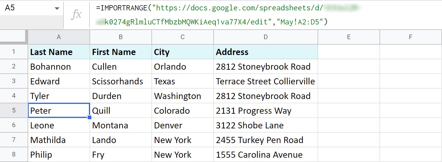
Using the Importrange function
If you have data spread across multiple Google Sheets and want to combine them into one, the Importrange function is a powerful tool to achieve this. With Importrange, you can fetch and import data from one sheet to another, allowing you to consolidate information from different sources.
Here’s how you can use the Importrange function:
1. Open the sheet where you want to import the data.
2. In an empty cell, start by typing the `=IMPORTRANGE` function.
3. Inside the parentheses, specify the source sheet’s URL enclosed in double quotes. For example:
`=IMPORTRANGE(“https://docs.google.com/spreadsheets/d/1234567890abcdefg/edit#gid=0”,`
4. After the URL, add a comma and enter the range or cell reference from the source sheet that you want to import. For example, if you want to import all the data from Sheet1, you would write:
`”Sheet1!A1:Z”`
5. Close the parentheses, and press Enter to import the data. Google Sheets may prompt you to grant access to the source sheet. Follow the instructions to allow access.
By using the Importrange function, you can bring in data from multiple sheets, even if they are in different workbooks. This is especially useful when you need to combine data from various team members or departments into a single sheet for analysis or reporting.
Keep in mind that the imported data is not linked, meaning any changes made in the source sheet will not automatically update in the destination sheet. You will need to manually refresh the function or use automation tools like Google Apps Script to automate the data fetching process.
Using the Importrange function in Google Sheets opens up a world of possibilities for aggregating and consolidating data. Whether you’re working on a personal project or collaborating with a team, this function will streamline the process and save you valuable time.
In conclusion, combining data in Google Sheets is an essential skill for anyone working with spreadsheet data. By using functions such as CONCATENATE, QUERY, or VLOOKUP, you can merge and manipulate data from different sources to gain valuable insights and streamline your analysis. With the ability to combine text, numbers, and formulas, Google Sheets provides a powerful platform for organizing and manipulating data in a user-friendly way. Whether you are a business analyst, a researcher, or a student, mastering the art of combining data in Google Sheets will greatly enhance your ability to make data-driven decisions and solve complex problems. So, don’t hesitate to explore the various techniques and features available in Google Sheets, and unlock the true potential of your data.
FAQs
1. Can I combine data from multiple sheets in Google Sheets?
Yes, you can combine data from multiple sheets in Google Sheets using various functions such as QUERY, IMPORTRANGE, or VLOOKUP. These functions allow you to pull data from different sheets and consolidate it into a single sheet.
2. How do I use the QUERY function to combine data in Google Sheets?
To use the QUERY function, you need to specify the range of data you want to combine and provide a query statement to filter and manipulate the data. The syntax for the QUERY function is as follows:
=query(‘Sheet1’!A1:Z, “SELECT *”)
This will pull all the data from Sheet1 and display it in the current sheet.
3. What is the IMPORTRANGE function in Google Sheets?
The IMPORTRANGE function allows you to import data from a different Google Sheet into your current sheet. To use this function, you need to specify the URL of the source sheet and the range of data you want to import. The syntax for the IMPORTRANGE function is as follows:
=IMPORTRANGE(“https://docs.google.com/spreadsheets/d/XXXXXX”, “Sheet1!A1:Z”)
4. Can I combine data from different tabs within the same Google Sheet?
Yes, you can combine data from different tabs within the same Google Sheet using functions like QUERY or IMPORTRANGE. These functions allow you to reference data from different tabs and merge them into a single sheet.
5. Are there any add-ons or plugins available to simplify the process of combining data in Google Sheets?
Yes, there are various add-ons and plugins available in the Google Workspace Marketplace that can help simplify the process of combining data in Google Sheets. Some popular ones include Advanced Find and Replace, Power Tools, and Merge Sheets. These tools provide additional functionalities and automation options to streamline the data combining process.