How To Format Phone Number In Google Sheets

Formatting phone numbers in Google Sheets can be a tricky task, but with the right techniques, it can be easily accomplished. Whether you are dealing with a list of contacts, sales data, or any other type of information that includes phone numbers, formatting them correctly is crucial for readability and analysis. In this article, we will explore different methods and formulas to properly format phone numbers in Google Sheets, ensuring consistency and accuracy in your data. Whether you have numbers with different formats or need to add area codes or country codes, we’ve got you covered. Stay tuned to find out how to effortlessly format phone numbers in Google Sheets and improve the organization and visual appeal of your data.

Inside This Article

1. Formatting Phone Numbers in Google Sheets
2. Method 1: Using the FORMAT function
3. Method 2: Using the TEXT function
4. Method 3: Using a custom formula
5. Method 4: Using the Find and Replace tool
6. Conclusion
7. FAQs

Formatting Phone Numbers in Google Sheets

Google Sheets is a powerful tool for managing data, and if you are working with phone numbers, it is essential to format them correctly. In this article, we will explore different formatting options for phone numbers in Google Sheets to ensure consistency and usability.

Formatting a Phone Number as Text

In some cases, you may want to keep the phone numbers in Google Sheets as simple text without any specific formatting. This can be useful when working with phone numbers that include special characters or non-standard formats. To format a phone number as text, follow these steps:

1. Select the cells containing the phone numbers that you want to format.
2. Right-click on the selected cells and choose “Format cells” from the menu.
3. In the “Number” tab, select “Plain text” as the format.
4. Click on the “Apply” button to apply the formatting.

Formatting a Phone Number with Parentheses

If you prefer a more traditional phone number format with parentheses around the area code, you can easily achieve this in Google Sheets. Here’s how:

1. Select the cells containing the phone numbers that you want to format.
2. Right-click on the selected cells and choose “Format cells” from the menu.
3. In the “Number” tab, select “Custom” as the format.
4. In the input box next to “Custom format”, enter the following:
   (###) ###-####
5. Click on the “Apply” button to apply the formatting.

Formatting a Phone Number with Dashes

In some cases, you may prefer to format the phone numbers with dashes between the digits for better readability. Here’s how you can achieve this format:

1. Select the cells containing the phone numbers that you want to format.
2. Right-click on the selected cells and choose “Format cells” from the menu.
3. In the “Number” tab, select “Custom” as the format.
4. In the input box next to “Custom format”, enter the following:
   ###-###-####
5. Click on the “Apply” button to apply the formatting.

Formatting a Phone Number with Country Code

If you are working with phone numbers that include country codes, you can format them accordingly in Google Sheets. Here’s how:

1. Select the cells containing the phone numbers that you want to format.
2. Right-click on the selected cells and choose “Format cells” from the menu.
3. In the “Number” tab, select “Custom” as the format.
4. In the input box next to “Custom format”, enter the following:
   +## ###-###-####
5. Click on the “Apply” button to apply the formatting.

By properly formatting phone numbers in Google Sheets, you can ensure consistency and improve the readability of your data. Whether you prefer a basic text format or want to include parentheses, dashes, or country codes, Google Sheets offers a variety of options to suit your needs. Take advantage of these formatting techniques to make your phone number data more organized and visually appealing.

Frequently Asked Questions

Q: Can I apply formatting to multiple cells at once in Google Sheets?

A: Yes, you can apply formatting to multiple cells by selecting them all at once and then applying the desired formatting from the “Format cells” menu.

Q: Can I change the format of phone numbers after they have been entered in Google Sheets?

A: Yes, you can change the format of phone numbers at any time by selecting the cells and applying the desired formatting from the “Format cells” menu.

Q: Will the formatting of phone numbers affect any calculations or formulas in Google Sheets?

A: No, the formatting of phone numbers does not affect any calculations or formulas in Google Sheets. The formatting is purely visual and does not alter the underlying data.

Q: Can I create my own custom phone number format in Google Sheets?

A: Yes, you can create your own custom phone number format by selecting “Custom” in the “Format cells” menu and entering the desired format in the input box.

Q: Can I remove the formatting of phone numbers in Google Sheets?

A: Yes, you can remove the formatting of phone numbers by selecting the formatted cells and choosing “Plain text” as the format from the “Format cells” menu.

Now that you know how to format phone numbers in Google Sheets, you can easily manage and present your data in the desired format. Experiment with different formats to find the one that suits your needs best and enhances the readability of your phone number data.

Method 1: Using the FORMAT function

One of the ways to format a phone number in Google Sheets is by using the FORMAT function. With this function, you can easily customize the appearance of your phone numbers in a specific format, such as adding parentheses or dashes.

To begin, let’s assume you have a phone number in cell A1 that you want to format. Here’s how you can use the FORMAT function:

1. Start by selecting an empty cell where you want the formatted phone number to appear.
2. Enter the following formula: =FORMAT(A1,"(###) ###-####"). Replace A1 with the cell reference that contains the phone number you want to format.
3. Press Enter to apply the formula and see the formatted phone number.

The “###” in the formula represents the digits of the phone number, while the parentheses and dashes are added as static characters. You can customize the format by modifying the formula accordingly. For example, you can use "###-###-####" if you prefer a different dash format.

Using the FORMAT function provides flexibility in formatting phone numbers in Google Sheets. You can easily adjust the format to match your preferred style or conform to specific requirements.

Method 2: Using the TEXT function

Another way to format phone numbers in Google Sheets is by using the TEXT function. This function allows you to format a cell value in a specified format.

Here’s how you can use the TEXT function to format phone numbers:

1. Start by selecting the cell where you want the formatted phone number to appear.

2. In the formula bar, type =TEXT(A1,"(###) ###-####"), replacing A1 with the cell reference that contains the phone number you want to format.

3. Press Enter to apply the formula and see the result.

The TEXT function uses a format code within quotation marks to specify the desired formatting. In the example above, the format code "(###) ###-####" formats the phone number with parentheses around the area code and a hyphen between the first three digits and the last four digits.

You can customize the format code to match the specific formatting you prefer. For example, if you want to format the phone number with dashes instead of parentheses, you can use the format code "###-###-####".

By using the TEXT function, you have the flexibility to format the phone number in various ways and customize it according to your preferences.

Method 3: Using a custom formula

If you prefer a more flexible approach to formatting phone numbers in Google Sheets, you can use a custom formula. This method allows you to specify the desired format and apply it to all the phone numbers in a column automatically.

To use a custom formula, follow these steps:

1. Select the column where the phone numbers are located.
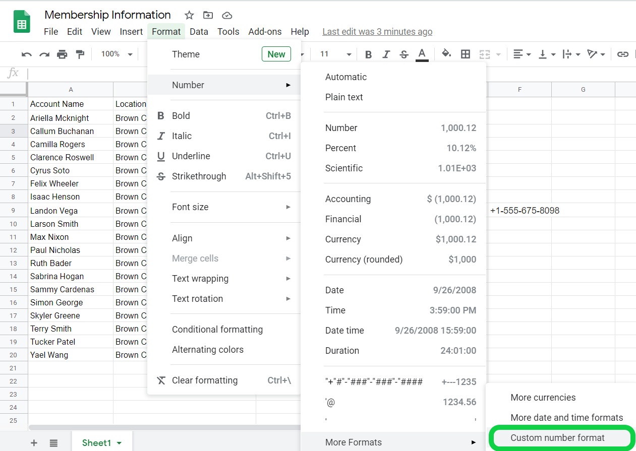
2. Click on the “Format” menu in the toolbar.
3. Choose “Number” and then “More formats” from the dropdown menu.
4. Select “Custom number format” at the bottom.
5. In the custom number format box, enter the desired format for the phone numbers.
6. Click on “Apply” to format the selected column with the custom formula.

For example, if you want to format the phone numbers in the column with parentheses and dashes (e.g., (123) 456-7890), you can use the following custom formula:

(###) ###-####

This formula will automatically format all the phone numbers in the selected column to match the specified pattern. You can customize the formula further by adding or removing parentheses, dashes, spaces, or any other characters as needed.

Using a custom formula allows you to quickly format phone numbers in Google Sheets without having to manually edit each entry. It provides a convenient way to ensure consistency and readability in your phone number data.

Keep in mind that the custom formula will only format the appearance of the phone numbers in the selected column. The underlying data will remain unchanged, making it easy to modify the formatting at any time without affecting the actual phone number values.

By utilizing the custom formula feature in Google Sheets, you have the flexibility to format phone numbers according to your specific requirements. Whether it’s adding parentheses, dashes, or any other formatting styles, you can easily apply them in bulk without the need for manual editing.

Method 4: Using the Find and Replace tool

If you are looking for a quick and efficient way to format phone numbers in Google Sheets, you can utilize the Find and Replace tool. This method allows you to replace certain characters or patterns in your data, making it ideal for reformatting phone numbers with ease.

Follow these steps to format phone numbers using the Find and Replace tool:

1. Open your Google Sheets document and navigate to the sheet containing the phone numbers that you want to format.
2. Select the range of cells that contain the phone numbers you wish to format. You can do this by clicking and dragging your cursor over the desired cells.
3. Click on “Edit” in the top menu bar, then select “Find and Replace.” Alternatively, you can use the keyboard shortcut “Ctrl + H” (Windows) or “Cmd + H” (Mac).
4. In the “Find” field, enter the specific character or pattern that you want to change. For example, if you want to remove parentheses from the phone numbers, enter “(” (without the quotes).
5. Leave the “Replace with” field empty if you want to remove the characters. If you want to replace the characters with something else, enter the desired replacement in the field.
6. Click on the “Replace” button to change the specific character or pattern in your selected range of cells.
7. Repeat steps 4-6 for any other characters or patterns you wish to change.

Using the Find and Replace tool gives you the flexibility to format phone numbers quickly and consistently in your Google Sheets document. Whether you need to remove parentheses, dashes, or any other characters, this method provides an efficient solution.

Remember to double-check your data after using the Find and Replace tool to ensure that the phone numbers are formatted correctly and without any unintended changes. This will help you maintain the accuracy and integrity of your data.

Conclusion

In conclusion, formatting phone numbers in Google Sheets is a simple and useful technique that can greatly enhance data organization and clarity. Whether you’re dealing with a list of customer contacts, a database of phone numbers, or any other data set that includes phone numbers, being able to format them correctly is essential. With the use of formulas, such as the regular expression formula, and custom formatting options, you can easily achieve the desired phone number format in Google Sheets.

By following the steps outlined in this article, you can ensure consistency, readability, and professionalism in your phone numbers. Properly formatted phone numbers not only make it easier to search and sort data but also improve the overall user experience. So, take the time to format your phone numbers in Google Sheets and enjoy the benefits of organized and well-presented data.

FAQs

1. How do I format a phone number in Google Sheets?
To format a phone number in Google Sheets, you can use a combination of functions and formatting options. First, select the cells containing the phone numbers that you want to format. Then, go to the “Format” menu and select “Number.” In the “Format Cells” sidebar, choose “Custom” and enter the desired phone number format. For example, you can use the format (123) 456-7890 for U.S. phone numbers.

2. Can I format phone numbers based on a specific country format?
Yes, Google Sheets allows you to format phone numbers based on specific country formats. If you have phone numbers from different countries in your spreadsheet, you can use the “Custom” format option and enter the format code accordingly. For instance, use +44 (0) 1234 567890 for UK phone numbers or +82-10-1234-5678 for South Korean phone numbers.

3. Can I format international phone numbers in Google Sheets?
Certainly! Google Sheets enables you to format international phone numbers based on the desired format. If you have phone numbers from different countries, you can use the “Custom” format option and input the format code. For example, you can use +1 (123) 456-7890 for U.S. phone numbers or +91 12345 67890 for Indian phone numbers.

4. How can I add dashes or other separators to phone numbers?
To add dashes or separators to phone numbers in Google Sheets, you can use a combination of functions and formatting options. First, select the cells with the phone numbers you want to modify. Then, go to the “Format” menu and select “Number.” In the “Format Cells” sidebar, choose “Custom” and enter the desired format. For instance, use 123-456-7890 for U.S. numbers or 12-3456-7890 for Japanese numbers.

5. Can I apply the phone number format to an entire column in Google Sheets?
Yes, you can easily apply the phone number format to an entire column in Google Sheets. To do this, click on the column letter to select the entire column. Then, follow the steps mentioned above to format the cells as phone numbers. The selected column will be formatted according to the chosen phone number format.