How To Pull Data From Another Tab In Google Sheets

Google Sheets is a powerful tool that allows you to organize and analyze your data. One of its key features is the ability to pull data from one tab to another. This functionality can streamline your workflow and make it easier to access and utilize information across different sheets.

Whether you’re working on a project, creating reports, or performing data analysis, pulling data from another tab in Google Sheets can save you time and ensure accuracy. In this article, we’ll explore the step-by-step process of pulling data from one tab to another and uncover some tips and tricks to enhance your productivity.

So, if you’re ready to unlock the full potential of Google Sheets and gain valuable insights from your data, let’s dive in and learn how to pull data from another tab in Google Sheets.

Inside This Article

1. Pulling Data from Another Tab in Google Sheets
2. Method 1: Using cell reference
3. Method 2: Using the IMPORTRANGE function
4. Method 3: Using the QUERY function
5. Conclusion
6. FAQs

Pulling Data from Another Tab in Google Sheets

Google Sheets is a powerful tool for organizing and analyzing data. One common task you may encounter is pulling data from another tab within the same Google Sheets document.

Accessing data within the same spreadsheet is relatively straightforward. All you need to do is reference the cell or range of cells in the specific tab where the data resides. For example, if you want to pull data from a tab called “Sales Data” in cell A2, you can simply use the formula “=Sales Data!A2” in the desired cell. This will display the value of cell A2 from the “Sales Data” tab in the current tab.

But what if you want to import data from a different spreadsheet altogether? Google Sheets allows you to do that as well. To import data from another spreadsheet, you need to use the “IMPORTRANGE” formula. This formula requires two parameters: the URL of the spreadsheet you want to import data from, and the range of cells you want to import.

For example, if you have a spreadsheet with the URL “https://docs.google.com/spreadsheets/d/your_spreadsheet_id/edit”, and you want to import cells A1 to C10 from the “Sheet1” tab, you would use the formula “=IMPORTRANGE(“https://docs.google.com/spreadsheets/d/your_spreadsheet_id/edit”, “Sheet1!A1:C10″)”.

The IMPORTRANGE formula will prompt you to grant permission for access to the external spreadsheet. Once you grant access, the imported data will be displayed in the current sheet.

Another handy feature in Google Sheets is the Query function, which allows you to pull and manipulate data based on specific criteria. The Query function can be used to extract data from another tab within the same spreadsheet.

For instance, if you have a tab called “Sales Data” with columns for date, product, and quantity, you can use the Query function to filter the data based on certain criteria. You can specify the range of data you want to query, along with the criteria you want to apply, and the Query function will provide you with the filtered results.

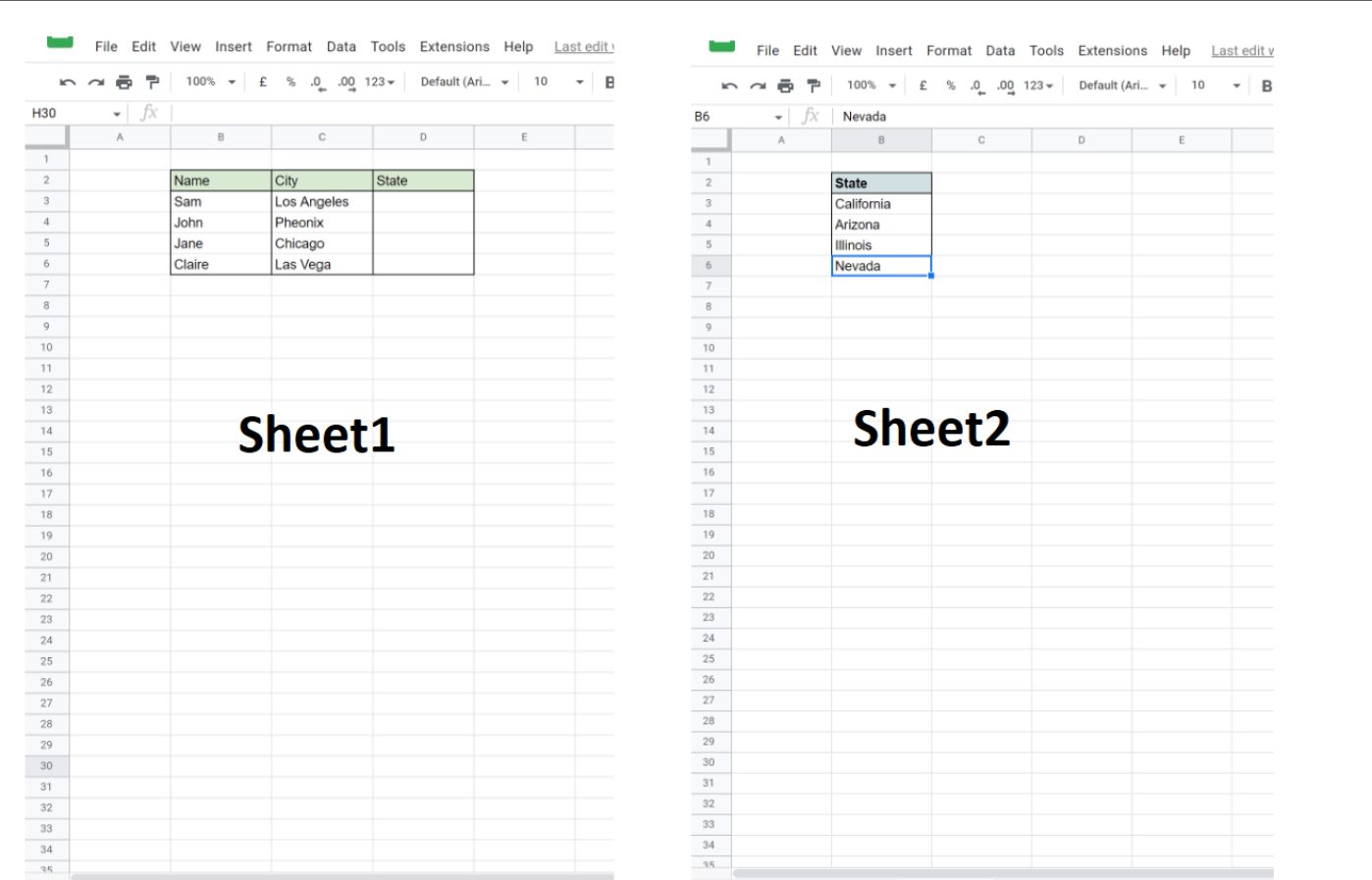
Method 1: Using cell reference

If you want to pull data from another tab in Google Sheets, one method is by using cell references. This allows you to directly reference a specific cell or range of cells from another sheet within the same spreadsheet.

To use this method, follow these steps:

1. Open the Google Sheets document that contains both the source tab (the tab you want to pull data from) and the destination tab (the tab you want to populate with the pulled data).
2. In the destination tab, select the cell where you want the data to appear.
3. Type an equals sign (=) in the selected cell to indicate that you’ll be using a formula.
4. Switch to the source tab and select the cell or range of cells you want to pull data from.
5. Return to the destination tab and you’ll notice that the cell reference for the selected cell(s) from the source tab has automatically appeared in the formula.
6. Press Enter to confirm the formula. The data from the source tab will now be displayed in the corresponding cell(s) of the destination tab.

Using cell references is a simple and efficient way to populate your sheets with data from another tab without duplicating the information. It’s particularly useful when you want to create a summary or aggregate data from multiple tabs within the same spreadsheet.

Method 2: Using the IMPORTRANGE function

A powerful and versatile formula in Google Sheets is the IMPORTRANGE function. This function allows you to pull data from a different tab or even a different spreadsheet into your current sheet. It is particularly useful when you need to consolidate data from multiple sources or collaborate with others.

The syntax for the IMPORTRANGE function is:

=IMPORTRANGE(spreadsheet_url, range_string)

The spreadsheet_url is the URL of the spreadsheet containing the data you want to import. The range_string specifies the cells or range of cells you want to import, using the A1 notation.

Before you can use the IMPORTRANGE function, make sure that you have the necessary permissions to access the source spreadsheet. Both the source and destination spreadsheets must be owned by you or shared with you with the necessary access permissions.

Here’s how you can use the IMPORTRANGE function to pull data from another tab:

1. Open your destination spreadsheet where you want the imported data to appear.

2. In an empty cell, enter the IMPORTRANGE formula, starting with an equals sign (=).

3. Inside the formula, provide the URL of the source spreadsheet surrounded by double quotes, followed by a comma (,).

4. Next, specify the range of cells you want to import from the source spreadsheet using the A1 notation, and close the formula with a closing parenthesis ).

5. Press Enter to apply the formula.

The IMPORTRANGE function will pull the data from the specified range in the source spreadsheet and display it in the destination spreadsheet. Any changes made to the source data will be reflected in real time in the destination spreadsheet, as long as you have the necessary permissions.

It’s important to note that when using the IMPORTRANGE function, the imported data is not editable in the destination spreadsheet. If you want to manipulate the data or perform additional calculations, you can use other functions or create references to the imported data in separate cells.

The IMPORTRANGE function is a powerful tool for gathering and consolidating data from multiple sources within Google Sheets. By mastering this function, you can save time and effort in managing and analyzing data across different tabs and spreadsheets.

Method 3: Using the QUERY function

Another way to pull data from another tab in Google Sheets is by utilizing the QUERY function. This function allows you to retrieve specific data from a range of cells, based on certain criteria or conditions.

The syntax of the QUERY function is:
QUERY(data, query, [header_row])

data: This refers to the range of cells or the name of the tab where the data is located. For example, if you want to pull data from a tab named “Sales,” you would enter “Sales” as the data parameter.

query: This is the query string, which defines the specific data you want to retrieve. You can use SQL-like syntax to filter the data, sort it, or apply conditions to it. For example, if you want to retrieve all the products with a price higher than $50, your query string would be “SELECT * WHERE B > 50.”

[header_row]: This is an optional parameter that specifies whether the data has a header row. If set to 1, it assumes the first row contains headers. If not provided, it defaults to 0, assuming there is no header row.

Here’s an example of how to use the QUERY function to pull data from another tab in Google Sheets:

1. First, select the cell where you want the data to be displayed.
2. Type the QUERY formula, starting with the equals sign (=).
3. Inside the formula, specify the range of cells or tab name where the data is located.
4. Next, add the query string to define the specific data you want to retrieve.
5. Press Enter, and the cells will display the requested data.

The QUERY function is highly flexible and allows you to perform complex data filtering and sorting operations. You can combine multiple conditions, use different logical operators, aggregate data, and more.

By using the QUERY function, you can easily extract and analyze data from multiple tabs within a Google Sheets document, providing you with powerful data manipulation capabilities.

In conclusion, learning how to pull data from another tab in Google Sheets can greatly enhance your productivity and streamline your workflow. By utilizing this feature, you can easily access and analyze data from different tabs within the same spreadsheet, eliminating the need for manual copying and pasting. This not only saves you time and effort but also reduces the risk of data errors.

Whether you are a student, a professional, or a small business owner, mastering this technique will empower you to organize and manipulate data more efficiently. By following the steps outlined in this article, you can confidently extract and display data from multiple tabs, allowing for a more comprehensive analysis and reporting.

So, why wait? Begin exploring this powerful feature today and discover how it can revolutionize the way you handle and analyze data in Google Sheets!

FAQs

1. Can I pull data from another tab in Google Sheets?

Yes, you can easily pull data from another tab in Google Sheets. Google Sheets allows you to reference data from different sheets within the same spreadsheet using formulas.

2. How do I pull data from another tab in Google Sheets?

To pull data from another tab in Google Sheets, you can use the =SheetName!A1 syntax. Replace “SheetName” with the name of the sheet you want to pull data from, and “A1” with the specific cell or range you want to retrieve the data from.

3. Can I pull data from multiple tabs in Google Sheets?

Yes, you can pull data from multiple tabs in Google Sheets by using the same formula syntax as mentioned above. Simply specify the name of the sheet followed by an exclamation mark, and then specify the cell or range from which you want to pull the data.

4. Can I update the pulled data automatically when the original data changes?

Yes, Google Sheets has a feature called “Automatic Update” that allows you to update the pulled data automatically when changes are made to the original data. By default, Google Sheets automatically recalculates the formulas when any changes occur.

5. Is it possible to pull data from a specific column or row in another tab?

Yes, you can pull data from a specific column or row in another tab by modifying the formula syntax. For example, to pull data from column B in the “Sheet2” tab, you would use the formula =Sheet2!B:B. Similarly, to pull data from row 3 in the “Sheet3” tab, you can use =Sheet3!3:3.