How To Add Color To Data Validation Google Sheets

Google Sheets is a powerful tool for managing and analyzing data, and one of its handy features is data validation. Data validation allows you to set rules and restrictions on the input values in your spreadsheet, ensuring that the data entered is accurate and consistent. While Google Sheets offers a variety of options for data validation, one aspect that can elevate the visual appeal of your spreadsheet is adding color. By adding color to the data validation rules, you can make it easier to identify and understand the different types of data being inputted. In this article, we will explore how to add color to data validation in Google Sheets, providing you with step-by-step instructions and useful tips to make your spreadsheets visually appealing and easy to navigate. So, let’s get started and unleash the vibrant potential of your data validation in Google Sheets!

Inside This Article

1. Understanding Data Validation in Google Sheets
2. Ways to Add Color to Data Validation
3. Step-by-Step Guide to Adding Color to Data Validation
4. Tips and Best Practices – Avoiding common mistakes when adding color to data validation – Optimizing the use of color to enhance data validation
5. Conclusion
6. FAQs

Understanding Data Validation in Google Sheets

Data validation is a powerful feature in Google Sheets that allows users to define a set of rules and restrictions for the data entered in a cell or range. It helps to ensure that the data is accurate, consistent, and within the specified parameters. By using data validation, you can prevent data entry errors and enforce data integrity in your spreadsheets.

Simply put, data validation acts as a gatekeeper for your data. It helps you control what can be entered into a cell or range, limiting it to specific values, numbers, dates, or even custom formulas. This ensures that your spreadsheet remains organized, error-free, and easy to use.

By implementing data validation in your Google Sheets, you can save time by reducing the need for manual data cleaning and validation. It also enhances the accuracy and reliability of your data, making it easier to analyze and present your findings.

Benefits of using Data Validation in Google Sheets

Data validation offers several benefits for users who work with Google Sheets:

1. Improved Data Accuracy: By restricting input to specific values or ranges, data validation helps to minimize human error and ensures that only valid and meaningful data is entered.
2. Consistency: Data validation allows you to enforce consistent data formats, such as dates, phone numbers, or email addresses, across multiple cells or ranges.
3. Data Integrity: By setting validation rules, you can prevent unwanted or invalid data from being entered into your spreadsheets, ensuring the integrity and reliability of your data.
4. Efficiency: With data validation, you can save time by preventing the need for manual data cleaning and validation. This allows you to focus on analyzing and utilizing the data rather than fixing errors.
5. User-Friendly Experience: Data validation can improve the usability of your spreadsheets by providing users with clear instructions and restrictions, making it easier for them to input data correctly.

Overall, data validation is a valuable tool for maintaining data accuracy, consistency, and integrity in Google Sheets. It allows you to create more reliable and user-friendly spreadsheets, ensuring that your data remains error-free and meaningful.

Ways to Add Color to Data Validation

Data validation is a powerful tool in Google Sheets that allows you to control the type and range of data that can be entered in a cell or range of cells. While data validation is primarily used to ensure data accuracy and consistency, you can also add a touch of visual appeal to your spreadsheets by incorporating color. Here are three options to add color to data validation in Google Sheets:

Option 1: Using conditional formatting with data validation

Conditional formatting is a feature in Google Sheets that allows you to apply formatting based on specific rules or conditions. By combining data validation with conditional formatting, you can highlight cells that meet certain criteria. To add color to data validation using conditional formatting, follow these steps:

1. Select the cells where you want to apply data validation.
2. Go to the “Data” menu and select “Data Validation.”
3. In the data validation dialogue box, choose the validation criteria and apply the desired settings.
4. Click on the “Format” tab in the dialogue box and select “Conditional formatting.”
5. Set the formatting rules to specify the desired color and style for the cells that meet the validation criteria.
6. Click “Save” to apply the data validation and conditional formatting.

With this option, you can visually distinguish cells that pass the data validation criteria from those that don’t, making it easier to identify valid data entries.

Option 2: Applying color rules based on data validation criteria

If you want more control over the specific color rules applied to your data validation, you can utilize the “Conditional Formatting” feature in Google Sheets. This allows you to create custom color rules based on the data validation criteria you have set. Here’s how:

1. Select the cells with data validation in your spreadsheet.
2. Go to the “Format” menu and choose “Conditional formatting.”
3. In the conditional formatting dialogue box, select the custom formula option.
4. Enter the formula that evaluates the data validation criteria and returns true or false.
5. Specify the formatting style, including the desired cell color, font color, etc.
6. Click “Save” to apply the conditional formatting based on the data validation criteria.

By customizing the conditional formatting rules, you can assign different colors to specific validation criteria, providing visual cues for different types of data entries.

Option 3: Using custom formulas with conditional formatting

If you want to take your data validation colorization to the next level, you can leverage the power of custom formulas in Google Sheets. Custom formulas allow you to define complex rules and conditions for applying colors to cells. Here’s how to use custom formulas with conditional formatting:

1. Select the range of cells to apply data validation and color rules.
2. Go to the “Format” menu and choose “Conditional formatting.”
3. In the conditional formatting dialogue box, select the custom formula option.
4. Enter the custom formula that evaluates the data validation criteria and returns true or false.
5. Specify the formatting style, including the desired cell color, font color, etc.
6. Click “Save” to apply the conditional formatting based on the custom formula.

With custom formulas, you have complete flexibility in defining the color rules based on your specific data validation requirements, allowing you to create visually appealing spreadsheets.

By utilizing these three options, you can add color to data validation in Google Sheets, making your spreadsheets not only functional and accurate but also visually appealing and easy to interpret.

Step-by-Step Guide to Adding Color to Data Validation

Are you looking to make your data validation in Google Sheets more visually appealing? Adding color to your data validation can make it easier to identify and interpret the information. In this step-by-step guide, we will walk you through the process of adding color to your data validation in Google Sheets. Let’s get started!

Step 1: Setting up the data validation in Google Sheets

The first step is to set up the data validation in your Google Sheets. Data validation allows you to define the rules and restrictions for the data entered in a specific range of cells. To set up data validation, follow these steps:

1. Select the range of cells where you want to apply the data validation.
2. Go to the “Data” menu and select “Data validation.”
3. In the data validation dialog box, choose the criteria for your data validation. This can include values from a list, numbers, dates, or custom formulas.
4. Specify any additional validation settings, such as allowing invalid entries or showing a warning message.
5. Click “Save” to apply the data validation to the selected range of cells.

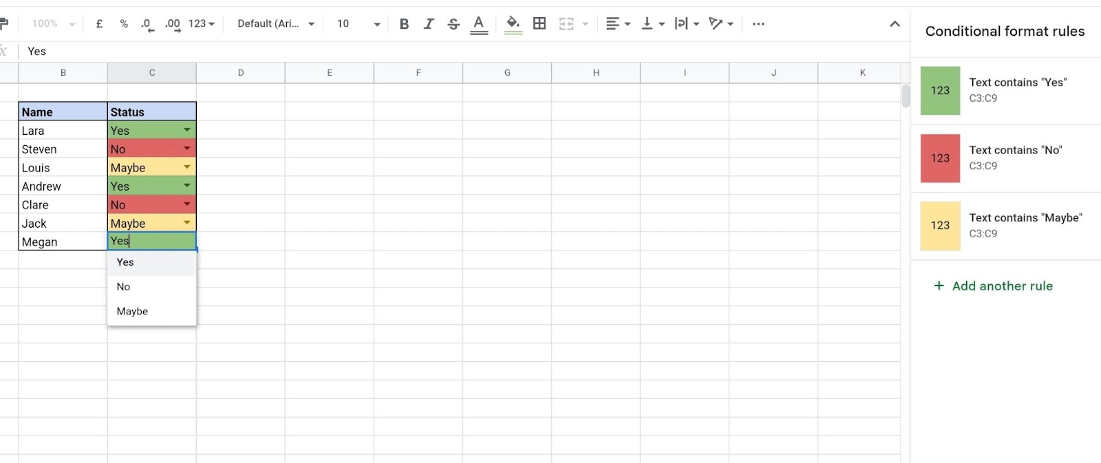
Step 2: Applying conditional formatting with color rules

Now that you have set up the data validation, you can apply conditional formatting with color rules to the cells. Conditional formatting allows you to automatically change the color of the cells based on certain criteria. Follow these steps to apply conditional formatting:

1. Select the range of cells where you want to apply the conditional formatting.
2. Go to the “Format” menu and select “Conditional formatting.”
3. In the conditional formatting dialog box, choose “Custom formula is” from the drop-down menu.
4. Enter the formula that will determine the color of the cells. This can be based on the value of the cell, the value in another cell, or a combination of values and operators.
5. Select the color you want to apply to the cells that meet the condition.
6. Click “Done” to apply the conditional formatting with color rules.

Step 3: Customizing colors based on data validation criteria

If you want to further customize the colors based on specific data validation criteria, you can use a combination of data validation rules and conditional formatting. Here’s how:

1. Edit the existing data validation rule or create a new one.
2. In the data validation dialog box, choose the criteria for your data validation.
3. Click on the “Conditional formatting” button.
4. Set up the conditional formatting rules and choose the colors for each rule.
5. Click “Done” to apply the customized colors to the data validation.

By following these steps, you can easily add color to your data validation in Google Sheets. This not only enhances the visual appeal of your spreadsheet but also helps you interpret and analyze the data more effectively. Take advantage of these customization options to make your data validation stand out!

Start applying color to your data validation today, and make your Google Sheets even more visually appealing and informative!

Tips and Best Practices – Avoiding common mistakes when adding color to data validation – Optimizing the use of color to enhance data validation

Adding color to data validation in Google Sheets can be a powerful way to make your data more visually appealing and easier to understand. However, it’s important to use colors judiciously and follow best practices to avoid common mistakes. Here are some tips to help you make the most of color in data validation:

1. Choose colors wisely: When adding color to your data validation, opt for colors that are easily distinguishable and don’t clash with the rest of your spreadsheet. It’s important to ensure that the colors you choose enhance the readability and clarity of your data, rather than creating confusion.

2. Use color sparingly: While color can be helpful in highlighting specific data, too much color can overwhelm the reader and make the information difficult to comprehend. Use color selectively and only where it adds value or draws attention to important insights.

3. Consider color-blindness: Keep in mind that not all users may be able to distinguish certain colors due to color vision deficiencies. Take into account different types of color blindness when selecting colors for your data validation. Consider using color schemes that are accessible to all users.

4. Use color to indicate meaning: One of the key benefits of adding color to data validation is that it can convey meaning without the need for lengthy explanations. Use color to represent different categories, highlight outliers, or indicate specific conditions. This can make it easier for users to interpret and analyze the data.

5. Maintain consistency: To avoid confusion, ensure that you use the same color palette consistently across your data validation. Consistency helps users quickly understand the meaning behind different colors and reduces the chance of misinterpretation or errors.

6. Test your color choices: Before finalizing your color scheme, it’s a good idea to test how it looks on different devices and screen resolutions. Colors may appear differently on different screens, so make sure your chosen colors maintain their legibility and effectiveness across different platforms.

7. Document your color choices: To maintain consistency and ensure clarity, document the color choices you have made for your data validation. This documentation can serve as a reference for yourself and others working with the spreadsheet, preventing confusion and potential discrepancies.

8. Regularly review and update: As your data or analysis requirements change, it’s important to review and update your color choices accordingly. Regularly reassess your use of color in data validation to ensure that it continues to meet your objectives and remains effective in conveying the intended message.

By following these tips and best practices, you can add color to data validation in Google Sheets in a way that enhances the readability and impact of your data. Remember to use colors thoughtfully and consistently, taking into account the needs and preferences of your audience. With the right approach, color can be a valuable tool for making your data more engaging and informative.

Conclusion

Adding color to data validation in Google Sheets is a powerful tool that can enhance the visual appeal and usability of your spreadsheets. By customizing the cell colors based on the validation criteria, you can quickly identify and analyze data trends, errors, or outliers. Whether you’re using dropdown lists, number ranges, or custom formulas, incorporating color coding can bring your data to life and make it easier to interpret.

With the step-by-step guide provided in this article, you now have the knowledge to implement color-coded data validation in your Google Sheets. Remember to use clear and meaningful colors that align with the validation rules for optimal clarity and understanding. By leveraging this feature effectively, you can elevate your data analysis capabilities and improve your overall spreadsheet experience.

So go ahead, give it a try and take your Google Sheets to the next level by adding color to your data validation!

FAQs

Here are some frequently asked questions about adding color to data validation in Google Sheets:

1. Can I add color to data validation in Google Sheets?

Yes, you can add color to data validation in Google Sheets. By using conditional formatting, you can set up rules that apply different colors to cells based on the validation criteria.

2. How do I add color to data validation in Google Sheets?

To add color to data validation in Google Sheets, follow these steps:

1. Select the range of cells you want to apply data validation to.
2. Go to the “Format” menu and choose “Conditional formatting.”
3. In the conditional formatting dialog box, choose “Custom formula is” under the “Format cells if” dropdown.
4. Enter the formula based on the validation criteria. For example, if you want to color cells with values greater than 10, you can enter the formula “=$A1>10” where A1 is the top-left cell of your selected range.
5. Select the formatting style and color you want to apply to the cells that meet the validation criteria.
6. Click “Done” to apply the formatting.

3. Can I apply multiple colors to data validation criteria in Google Sheets?

Yes, you can apply multiple colors to data validation criteria in Google Sheets. By setting up multiple conditional formatting rules, each with a different criteria and color, you can achieve this. For example, you can have a rule that colors cells with values greater than 10 in green, and another rule that colors cells with values less than 5 in red.

4. How do I edit or remove color from data validation in Google Sheets?

To edit or remove color from data validation in Google Sheets, follow these steps:

1. Select the range of cells with the existing data validation formatting.
2. Go to the “Format” menu and choose “Conditional formatting.”
3. In the conditional formatting dialog box, you can either edit the existing rule by clicking on it or remove the rule by clicking on the trash bin icon next to it.
4. Make the necessary changes or click “Done” to remove the rule.

5. Can I apply color to data validation based on a list of values in Google Sheets?

Yes, you can apply color to data validation based on a list of values in Google Sheets. By setting up a conditional formatting rule using the formula “=$A1={“Value 1″,”Value 2″,”Value 3″,…}” where A1 is the top-left cell of your selected range, you can apply different colors to cells that match the values in the list.