
Are you looking to create a graph in Google Sheets using two sets of data? Whether you need to visualize trends, compare data, or showcase patterns, Google Sheets provides a user-friendly platform for generating professional and informative graphs.
From line graphs to bar graphs, Google Sheets offers a variety of chart types to effectively present your data. By incorporating multiple data sets into a single graph, you can easily compare and analyze different variables.
In this article, we will guide you through the process of creating a graph in Google Sheets with two sets of data. Follow the step-by-step instructions and unleash the power of data visualization to gain valuable insights.
Inside This Article
- Overview
- Step 1: Open Google Sheets
- Step 2: Enter your data into the spreadsheet
- Step 3: Select the data range for the first set of data
- Step 4: Create a chart using the first set of data
- Step 5: Select the data range for the second set of data
- Step 6: Add the second set of data to the chart
- Step 7: Customize the graph
- # 7.1 Adjusting the chart type
- # 7.2 Changing the chart title and axis labels
- 3 Formatting the data series
- Step 8: Finalize and save your graph
- Additional Tips and Tricks
- # Tip 1: Using a secondary axis
- # Tip 2: Adding a trendline
- Conclusion
- FAQs
Overview
If you’re looking to create a graph in Google Sheets with two sets of data, you’ve come to the right place! Google Sheets is a powerful tool for data analysis and visualization, and it offers a variety of options for creating graphs and charts.
In this article, we will walk you through the step-by-step process of making a graph in Google Sheets using two sets of data. Whether you’re comparing sales figures, tracking trends, or analyzing data sets, creating a graph can help you visualize the information and gain insights.
By following this guide, you’ll learn how to enter your data into a spreadsheet, select the appropriate data ranges, create a chart, and customize it to your liking. We’ll also provide some additional tips and tricks to take your graph-making skills to the next level.
So, let’s dive in and discover how to effectively make a graph in Google Sheets with two sets of data!
Step 1: Open Google Sheets
Before you can begin creating a graph in Google Sheets with two sets of data, you need to open Google Sheets on your computer or mobile device. Google Sheets is a free, web-based spreadsheet program that allows you to create, edit, and share spreadsheets online.
To open Google Sheets, follow these simple steps:
- Open your web browser.
- Type “sheets.google.com” into the address bar.
- Press Enter or Return on your keyboard.
- If you have a Google account, sign in. If you don’t have a Google account, you can create one for free by clicking on the “Create account” button.
- Once you’re signed in, you’ll be taken to the Google Sheets homepage.
Now that you’ve successfully opened Google Sheets, you’re ready to move on to the next step of creating a graph with two sets of data.
Step 2: Enter your data into the spreadsheet
Now that you have opened Google Sheets and are ready to create your graph, you need to enter your data into the spreadsheet. This step is crucial as it forms the foundation of your graph.
Start by identifying the variables you want to compare and organize them into columns. For example, if you are comparing sales data for different months, you would create one column for the months and another for the corresponding sales numbers.
To enter the data, simply click on the first cell in the appropriate column and start typing. You can use the arrow keys to move to the next cell or press the ‘Tab’ key to automatically move to the cell in the same row in the next column. You can also use the ‘Enter’ key to move to the cell below.
If you already have your data in another file or document, you can copy and paste it into Google Sheets. To do this, select the cells containing the data, use the ‘Ctrl+C’ (or ‘Command+C’ on Mac) shortcut to copy it, then go to the desired cell in Google Sheets and use the ‘Ctrl+V’ (or ‘Command+V’ on Mac) shortcut to paste the data.
Continue entering your data until you have populated all the necessary cells. Take your time to ensure accuracy and double-check your entries. Incorrect or incomplete data can lead to inaccurate or misleading graphs.
Once you have entered your data, you are ready to move on to the next step: selecting the data range for the first set of data.
Step 3: Select the data range for the first set of data
In order to create a graph in Google Sheets with two sets of data, you first need to select the data range for each set. For the first set of data, follow these steps:
- 1. Open your Google Sheets document and navigate to the sheet where your data is stored.
- 2. Identify the range of cells that contain the first set of data.
- 3. Click and drag your cursor to select the entire range of cells for the first set of data.
It’s important to ensure that you include all the necessary data points for accurate representation in your graph. Be sure to select only the cells that contain the relevant data and exclude any extra rows or columns.
Once you have selected the data range for the first set, you are ready to move on to the next step of creating your graph!
Step 4: Create a chart using the first set of data
Now that you have entered your data into the Google Sheets spreadsheet, it’s time to create a chart using the first set of data. This will help you visualize and analyze the information in a more meaningful way. Follow the steps below to create a chart:
- Select the data range for the first set of data:
To create a chart, you need to select the range of cells containing the data you want to include in the chart. Click and drag to select the cells that correspond to the first set of data. Make sure to include both the labels and the values. - After selecting the data range, click on the “Insert” tab in the menu at the top of the Google Sheets window. You will see a variety of chart options available to choose from.
- Click on the chart type that best suits your needs. Google Sheets offers a range of chart options including line charts, bar graphs, pie charts, and more.
- Once you have selected the chart type, Google Sheets will automatically generate a chart based on the selected data range. The chart will appear within the spreadsheet, allowing you to view and customize it as needed.
This step is crucial in visually representing your data, allowing you to easily identify patterns, trends, and outliers. Whether you want to compare different data sets or track changes over time, creating a chart using the first set of data can significantly enhance your analysis.
By following these simple steps, you can create a chart using the first set of data in Google Sheets. Remember, charts provide a visual representation of your data, making it easier to understand and interpret the information. So go ahead, start creating your chart and unlock valuable insights from your data!
Step 5: Select the data range for the second set of data
Now that you have created a chart using the first set of data, it’s time to add the second set of data to your graph. This will allow you to visualize the relationship or comparison between the two sets of data.
To select the data range for the second set of data, navigate back to your Google Sheets spreadsheet. Look for the column or columns that contain the data you want to plot on the graph alongside the first set of data. Once you have identified the appropriate columns, click and drag to highlight the cells that correspond to the second dataset.
For example, if your first set of data is located in column A and your second set of data is in column B, you would click and drag to select the cells in column B that contain the data you want to include in the graph.
It’s important to note that the selected range for the second set of data should have the same number of rows as the first set of data. This ensures that the data points align correctly on the graph.
Once you have selected the appropriate data range for the second set of data, you are ready to proceed to the next step and add it to your graph.
Step 6: Add the second set of data to the chart
Now that you have created the initial chart using the first set of data, it’s time to add the second set of data to the graph. This will allow you to compare and visualize the relationship between the two sets of data.
To add the second set of data, you will need to select the existing chart. Once selected, look for options to edit or modify the chart. In Google Sheets, this can usually be done by clicking on the chart area or using the “Edit” button that appears when the chart is selected.
After entering the chart editing mode, locate the option to add or modify the data range. In Google Sheets, this is typically found in the chart editor toolbar or under a “Data” or “Series” tab. Select the second data range and confirm your selection.
Once the second data set is added, you should see the corresponding data points appear on the chart. The chart will now reflect the relationship between both sets of data, allowing you to evaluate and analyze their correlations.
Keep in mind that it is important to ensure the accuracy and appropriateness of the data range you select for the second set. Make sure the data sets align with the intended purpose of your graph and effectively convey the message you want to convey.
Step 7: Customize the graph
Once you have created your graph using the first set of data, you can proceed to customize it further to make it more visually appealing and informative. Customizing the graph allows you to highlight specific data points, adjust the chart type, and add labels and titles. Here are some key options for customizing your graph:
7.1 Adjusting the chart type: Google Sheets offers a variety of chart types to choose from, including bar graphs, line graphs, pie charts, and more. You can experiment with different chart types to find the one that best represents your data. To change the chart type, simply click on the “Chart type” drop-down menu in the Chart editor toolbar and select your desired type.
7.2 Changing the chart title and axis labels: You can customize the chart title and axis labels to provide a clear explanation of what the graph represents. To edit the chart title, click on it and type in your desired text. Similarly, you can select the axis labels and modify them according to your requirements.
7.3 Formatting the data series: If you have multiple data sets in your graph, you can format each series individually to differentiate them visually. By selecting a specific data series, you can change its color, adjust the line thickness, and add different marker styles. This helps to highlight specific trends or patterns within the data.
Remember to save your changes periodically as you customize the graph to ensure that your modifications are retained. By taking the time to customize your graph, you can create a visually appealing representation of your data that effectively communicates the insights you wish to convey.
# 7.1 Adjusting the chart type
One of the great features of creating a graph in Google Sheets is the ability to adjust the chart type to best represent your data. Google Sheets offers a wide range of chart types, each with its own strengths and purposes. Let’s explore how to adjust the chart type to ensure your graph effectively communicates your data.
To begin, select the chart you created using the steps outlined in the previous sections. Once the chart is selected, you will notice a small chart icon in the top right corner. Clicking on this icon will open the “Chart editor” sidebar.
In the “Chart editor” sidebar, you will find various customization options, including the “Chart type” section. Here, you can choose from a variety of chart types such as bar charts, line charts, pie charts, and more. Simply click on the dropdown menu and select the desired chart type that best suits your data.
Each chart type has its own unique visual representation and is best suited for specific types of data. For example, a bar chart is ideal for comparing different categories, while a line chart is more suitable for showcasing trends over time.
Experiment with different chart types to see which one provides the clearest and most impactful visual representation of your data. You can instantly preview how your data will look in different chart types by selecting the desired option and observing the changes in the chart preview.
It’s important to choose a chart type that not only effectively communicates your data but also aligns with the overall aesthetics and message you want to convey. The right chart type can greatly enhance the impact of your graph and make it more engaging for your audience.
Once you have selected the appropriate chart type, you can further customize the graph by adjusting other settings such as colors, fonts, and layout. This will allow you to create a visually appealing and informative graph that effectively conveys your data.
Remember, the goal of adjusting the chart type is to enhance the clarity and understanding of your data. Take the time to consider the nature of your data and the story you want to tell so that you can choose the best chart type to effectively communicate your message.
# 7.2 Changing the chart title and axis labels
Once you have created your graph in Google Sheets, you can easily customize it by changing the chart title and axis labels. This allows you to provide clear and descriptive information to your audience, making your graph more informative and visually appealing.
To change the chart title, simply click on the existing title and type in your desired title. You can be creative with your chart title, making it catchy and attention-grabbing. Consider using keywords to make it relevant to your data and to attract readers’ interest.
Similarly, modifying the axis labels can provide additional context and clarity to your graph. You can change the labels for both the x-axis (horizontal) and the y-axis (vertical) to reflect the data you are displaying. For example, if you are plotting sales data over time, you can label the x-axis as “Months” and the y-axis as “Sales Amount.”
Google Sheets also allows you to customize the font style, size, and color of the chart title and axis labels. You can do this by selecting the text and using the formatting options provided in the toolbar. Experiment with different font styles and colors to find the combination that best suits your graph and makes it visually appealing.
Remember, the chart title and axis labels play an important role in communicating the purpose and meaning behind your graph. Take the time to choose clear and concise labels that effectively convey the information you want to present.
By customizing the chart title and axis labels in Google Sheets, you can make your graph more engaging and informative. This allows you to present your data in a visually appealing manner, capturing your audience’s attention and effectively conveying your message.
3 Formatting the data series
Once you have created a chart and added your data sets, you can further enhance the visual representation by formatting the data series. This allows you to customize the appearance of each set of data in your graph.
To format the data series in Google Sheets, follow these steps:
Step 1: Click on the chart to select it.
Step 2: In the chart editor panel on the right side of the screen, click on the “Customize” tab.
Step 3: Under the “Series” section, you will see a list of the data series in your chart.
Step 4: Click on the data series that you want to format. The formatting options for that series will appear.
Step 5: Customize the formatting options according to your preferences. You can modify the color, style, and other visual aspects of the data series.
Step 6: Repeat the process for any other data series that you want to format.
By formatting the data series, you can differentiate between different sets of data or highlight specific data points. This can make your graph more visually appealing and easier to understand.
Remember to maintain consistency in your formatting choices to ensure a cohesive and professional-looking graph.
Once you are satisfied with the formatting of your data series, click on the “Apply” or “Done” button to finalize the changes and update your graph.
Continue to experiment with different formatting options to find the style that best suits your needs. You can always go back and make adjustments to the formatting as required.
Pro tip: If you have multiple data series and want to apply the same formatting to all of them, you can select the first series, apply the desired formatting, and then use the “Copy formatting” option to apply it to the other series.
With the ability to format data series in Google Sheets, you can create visually stunning graphs that effectively convey your data and insights.
Step 8: Finalize and save your graph
Once you have created and customized your graph in Google Sheets, it’s time to finalize and save it. Follow these steps to complete the process:
1. Take a final look at your graph and make any necessary adjustments. Check that all the data points are accurate and labeled correctly. You can use the various customization options mentioned in the previous steps to fine-tune the appearance of your graph.
2. Check the axes and ensure that they are labeled appropriately. You want your audience to understand the data easily, so make sure the axis labels are clear and concise. If needed, modify the font size or orientation to increase readability.
3. Double-check the chart title. The title should effectively summarize the information presented in the graph. Make sure it accurately reflects the purpose of your graph and adds value to your audience’s understanding.
4. Adjust the chart’s visual elements, such as colors, fonts, and backgrounds, to match your desired style. You can experiment with different options until you achieve the desired visual aesthetic.
5. Once you are satisfied with the final look of your graph, it’s time to save it. Click on the “File” menu in Google Sheets and select “Download” to save the graph as an image file (e.g., PNG or JPEG). Choose a location on your computer to save the file.
6. Alternatively, you can also directly insert the graph into a Google Docs or Google Slides presentation. Simply click on the “Insert” menu, select “Chart,” and choose the desired graph from your saved Sheets document. This option allows you to easily update the graph if the data in the spreadsheet changes.
7. Finally, if you want to share your graph with others, you can generate a shareable link or provide them with access to the Google Sheets document itself. This way, viewers can interact with the graph or refer back to it whenever needed.
By following these steps, you can finalize and save your graph in Google Sheets, ensuring that it looks visually appealing, accurately represents your data, and effectively conveys your message to your intended audience.
Additional Tips and Tricks
When it comes to creating graphs in Google Sheets with two sets of data, there are a few additional tips and tricks that can help you enhance your visualizations. Let’s explore some of these advanced techniques:
Tip 1: Using a secondary axis
In some cases, you may have two sets of data with significantly different scales or units of measurement. To avoid the overlap and ensure clarity, you can use a secondary axis to represent one of the data sets on a separate scale. This allows viewers to easily compare both sets of data without any confusion.
To utilize a secondary axis, follow these steps:
- Select the data series that you want to represent on the secondary axis.
- Right-click on the selected data series and choose “Series” from the options.
- In the “Axis” section, select “Secondary Axis”.
- Click on “Apply” to add the data series to the secondary axis.
Tip 2: Adding a trendline
If you want to visualize the trend or pattern of your data, you can add a trendline to your graph. A trendline helps you identify any increasing or decreasing trend in your data points. This is particularly useful when analyzing data over time or when trying to identify correlations between variables.
To add a trendline, follow these steps:
- Select the data points for which you want to add a trendline.
- Click on the “Chart Elements” button (plus icon) on the right side of the chart.
- Check the “Trendline” option.
- Choose the type of trendline you want to add, such as linear, exponential, or polynomial.
Experiment with different trendline types to find the one that best represents your data.
By incorporating these tips and tricks into your graph-making process, you can create visually appealing and informative charts in Google Sheets that effectively convey your data. Remember to play around with customization options and experiment with different chart types to find the perfect visualization for your specific needs.
Now that you have learned how to create a graph in Google Sheets with two sets of data, it’s time to put your newfound skills to use and start visualizing your own data!
# Tip 1: Using a secondary axis
When creating a graph in Google Sheets with two sets of data that have different scales or units of measurement, it can be helpful to use a secondary axis. This allows you to clearly visualize the relationship between the two sets of data, even if they have vastly different values.
To use a secondary axis in Google Sheets, follow these steps:
- Select your chart by clicking on it.
- Click on the “Customize” tab in the right sidebar.
- Scroll down and locate the “Axes” section.
- Toggle the switch next to “Use Secondary Axis” to enable it.
Once the secondary axis is enabled, you will notice that one of the data series shifts to the right side of the graph, indicating that it is now associated with the secondary axis. This allows you to compare the data more accurately, without the values being distorted due to differing scales.
Why is using a secondary axis useful?
Using a secondary axis is particularly useful when dealing with data sets that have different units of measurement. For example, if you are comparing sales revenue with the number of units sold, the revenue will typically be much larger than the number of units. By using a secondary axis, you can ensure that both sets of data are clearly displayed without any loss of information.
Benefits of using a secondary axis:
- Allows for accurate comparison of data with different scales.
- Prevents distortion or loss of information.
- Enables you to easily identify any trends or patterns in the data.
Keep in mind:
While using a secondary axis can be beneficial, it’s important to use it responsibly and avoid misleading interpretations. Be sure to clearly label each axis and provide a clear explanation of the data sets being compared. Additionally, make sure to choose an appropriate chart type that effectively represents the relationship between the data.
By utilizing the secondary axis feature in Google Sheets, you can create visually appealing and informative graphs that accurately represent the relationship between two sets of data.
# Tip 2: Adding a trendline
Adding a trendline to your graph can provide valuable insights into the data trends and help you make more accurate predictions. Google Sheets offers a simple and powerful feature to add trendlines to your graphs. Here’s how you can do it:
1. Select your graph by clicking on it. You should see a small toolbar appear at the top right corner of your graph.
2. Click on the three-dot icon on the toolbar and select “Edit chart” from the dropdown menu.
3. In the Chart editor pane that appears on the right side of your screen, navigate to the “Customize” tab. Here, you’ll find various customization options.
4. Scroll down until you find the “Trendline” section. Enable the “Show trendline” option by checking the box next to it.
5. Once you’ve enabled the trendline, you can choose the type of trendline you want to add. Google Sheets offers several options, including linear, exponential, logarithmic, and more. Select the type that best suits your data.
6. You can further customize the trendline by adjusting the color, thickness, and style. Take a moment to experiment and find the visual representation that works best for your graph.
7. After customizing the trendline, click the “Apply” button to make the changes take effect.
Adding a trendline to your graph can help you identify patterns, correlations, and future projections in your data. It enhances the visual representation of your data and makes it easier for viewers to interpret the trends. Whether you’re analyzing sales trends, stock market data, or any other dataset, adding a trendline can provide valuable insights and improve decision-making.
So, take advantage of this powerful feature in Google Sheets and make your graphs more informative and visually appealing by adding trendlines.
In conclusion, creating a graph in Google Sheets with two sets of data is a simple and effective way to visually represent and analyze your data. By following the steps outlined in this article, you can easily plot your data points and customize the graph to suit your needs.
Google Sheets offers a wide range of graph types and customization options, allowing you to create professional-looking charts with ease. Whether you’re comparing sales figures, tracking trends over time, or analyzing survey responses, utilizing graphs can provide valuable insights into your data.
With its user-friendly interface and powerful features, Google Sheets is a versatile tool for data analysis and visualization. By mastering the art of creating graphs with two sets of data, you can unlock the full potential of Google Sheets and make meaningful interpretations of your data.
FAQs
1. Can I create a graph in Google Sheets with two sets of data?
Yes, you can create a graph in Google Sheets using two sets of data. Google Sheets provides various options to visualize data, including line graphs, bar graphs, pie charts, and more. By selecting the appropriate chart type and inputting both sets of data, you can easily create a graph that represents the relationship between the two sets of data.
2. How do I input two sets of data in Google Sheets?
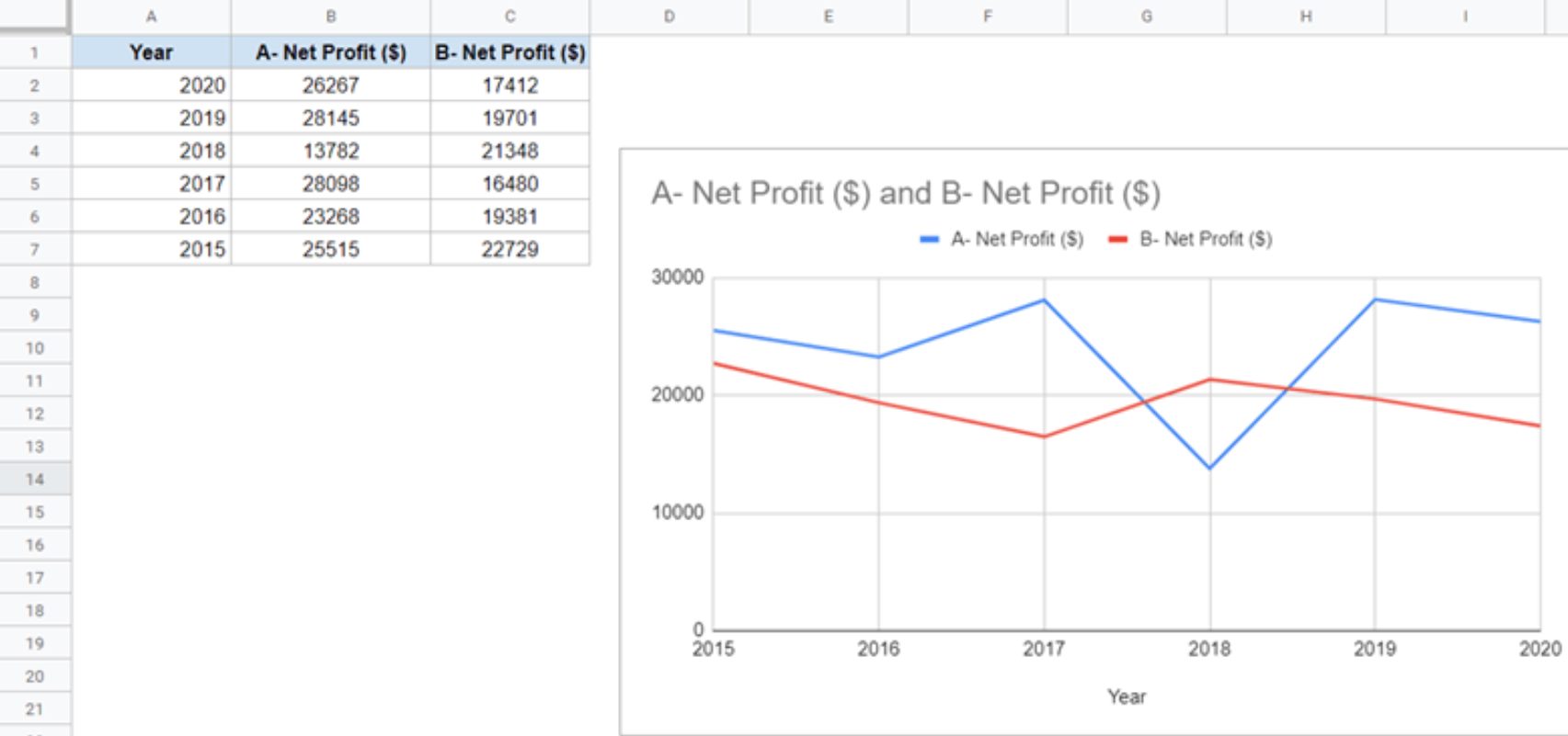
To input two sets of data in Google Sheets, you need to first open a new or existing spreadsheet. Enter your data in separate columns or rows. For example, if you have two sets of data in columns A and B, with each set having corresponding values in rows 2 to 10, you would enter the first set in column A and the second set in column B. This allows you to easily reference and visualize the data together.
3. Which chart type should I use for displaying two sets of data?
The choice of chart type depends on the nature of your data and what you would like to emphasize. Line graphs are often used to show trends over time or to compare two sets of data. Bar graphs are suitable for comparing different categories with two sets of data. Scatter plots can be used to show the relationship between two variables. Consider your data and the story you want to tell with your graph to choose the most appropriate chart type.
4. How can I customize the appearance of the graph in Google Sheets?
Google Sheets allows you to customize the appearance of your graph in various ways. You can change the colors, fonts, axes labels, legend, and many other visual aspects. Simply select the graph and click on the ‘Edit Chart’ option that appears. From there, you can access a variety of customization options that allow you to personalize the look of your graph to suit your preferences or match your branding.
5. How can I share the graph created in Google Sheets with others?
To share the graph created in Google Sheets with others, you can use the built-in sharing functionality. Click on the ‘Share’ button in the top-right corner of the Google Sheets interface. From there, you can enter the email addresses of the people you want to share the graph with and choose the level of access they have (view only, comment, or edit). This makes it easy to collaborate and share your graph with colleagues, clients, or anyone you wish to communicate your data to.