
In today’s data-driven world, visual representations are often the most effective way to convey complex information. Excel, with its powerful data analysis capabilities, is a popular tool for creating graphs and charts. One common requirement is to create a graph with multiple data sets, allowing for easy comparison and analysis. But how exactly can you make an Excel graph with multiple data sets?
In this article, we will guide you through the step-by-step process of creating an Excel graph with multiple data sets. We will explore different types of graphs that are best suited for displaying multiple data sets and provide tips on how to organize your data for optimal results. Whether you need to present sales data, market trends, or scientific research findings, knowing how to create an Excel graph with multiple data sets will help you effectively communicate your information in a visually appealing and easy-to-understand manner.
Inside This Article
- Formatting the Data Sets
- Selecting the Graph Type
- Creating the Graph
- Customizing the Graph Appearance
- Conclusion
- FAQs
Formatting the Data Sets
When creating a graph with multiple data sets in Excel, it is crucial to format the data sets properly to ensure accuracy and clarity in your graph. Follow these steps to format the data sets effectively:
1. Organize and Label the Data: Start by organizing your data into columns or rows. Each column or row should represent a different data set. It’s important to label each data set clearly so that it can be easily identified in the graph.
2. Remove Blank Cells: Check for any blank cells within the data sets and remove them. Blank cells can disrupt the graph and lead to inaccuracies in the visualization.
3. Apply Consistent Formatting: Ensure that each data set is formatted consistently. This includes using the same units, number formats, and date formats across all data sets. Consistent formatting will make it easier for viewers to interpret the graph accurately.
4. Sort the Data: If necessary, sort the data sets in ascending or descending order to create a more meaningful graph. Sorting the data sets can highlight trends and patterns to make the graph more informative.
5. Check for Data Errors: Review the data sets for any errors, such as incorrect values or missing data. Correct any errors before creating the graph to ensure accurate representation.
6. Calculate Additional Data Points: If needed, calculate any additional data points that are not already included in the data sets. These calculated data points can be added to the graph to provide more comprehensive insights.
By following these steps to format the data sets properly, you will be well on your way to creating an Excel graph with multiple data sets that is accurate, clear, and visually appealing.
Selecting the Graph Type
When it comes to creating an Excel graph with multiple data sets, selecting the right graph type is crucial for effectively visualizing your data. Excel offers a variety of graph types, and choosing the most appropriate one can greatly enhance the overall presentation and understanding of your data.
The selection of the graph type depends on the nature of your data and the insights you want to convey. Here are a few popular graph types to consider when working with multiple data sets:
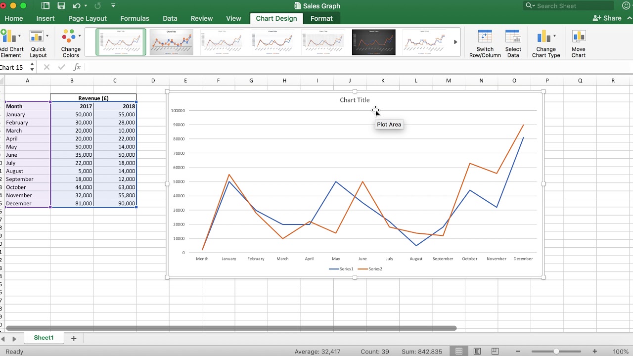
- Line Graph: A line graph is ideal for showing trends over a continuous interval of time or representing data with continuous variables. It is commonly used to track changes over time or to compare multiple data sets. Each data set is represented by a distinct line, making it easy to compare their progressions.
- Bar Graph: A bar graph is useful when comparing discrete data categories or data sets that are not continuous. Each data set is represented by a separate bar, and the height of the bar represents the value of the data. This allows for quick visual comparison between different data sets.
- Pie Chart: A pie chart is suitable for showing the proportion and distribution of different data sets or categories. Each data set is represented by a “slice” of the pie, with the size of the slice reflecting the proportion of that data set. Pie charts work best when dealing with a small number of data sets.
- Scatter Plot: A scatter plot is effective for visually showing the relationship between two continuous variables. Each data point on the graph represents a combination of values from the two variables, and the position of the point on the graph provides insights into their correlation.
These are just a few examples of graph types available in Excel. Ultimately, the choice of graph type should align with your specific data and the story you want to tell. Experiment with different graph types to find the one that best represents your data and helps you make the most compelling visualizations.
“
Creating the Graph
Once you have formatted your data sets and selected the appropriate graph type, it’s time to create your graph in Excel. Follow these simple steps to bring your data to life:
1. Highlight the data sets you want to include in your graph. To do this, click and drag your cursor over the cells containing the data. Make sure to include the appropriate labels for the x-axis and y-axis.
2. With your data selected, navigate to the ‘Insert’ tab in the Excel ribbon. Here, you will find various graph types such as bar graphs, line graphs, pie charts, and more. Choose the graph type that best represents your data and click on it.
3. A basic graph will be inserted into your Excel worksheet. This graph will display your selected data sets in a default format. Don’t worry, as you can easily customize the appearance of your graph in the next step.
4. Use the ‘Chart Elements’ and ‘Chart Styles’ options in the Excel ribbon to customize your graph. You can add titles, labels, gridlines, legends, and more. Experiment with different styles and layouts until you achieve the desired look.
5. If you want to further customize your graph, double-click on specific elements within the graph to access additional formatting options. This allows you to change colors, fonts, data labels, and other visual elements to make your graph more visually appealing and informative.
6. Finally, once you are satisfied with the appearance of your graph, you can save it, print it, or copy and paste it into other applications or documents.
Creating a graph in Excel with multiple data sets is a straightforward process. By following these steps and utilizing the customization options available, you can create visually compelling graphs that effectively convey your data.”
Customizing the Graph Appearance
Once you have created a graph in Excel with multiple data sets, you may want to customize its appearance to make it more visually appealing and easier to understand. Luckily, Excel offers several options for customizing the graph’s appearance to suit your needs.
1. Axis Labels and Titles: Axis labels and titles provide crucial information about the data being represented. You can customize the labels and titles by right-clicking on the axis or title and selecting the “Format Axis” or “Format Title” option. From there, you can modify the font, size, color, and alignment of the labels and titles.
2. Data Labels: Data labels help identify individual data points on a graph. You can choose to display data labels for each data series or specific data points. To customize the data labels, right-click on a data point and select the “Add Data Labels” option. You can then modify the appearance and position of the data labels as desired.
3. Chart Styles: Excel provides a range of pre-defined chart styles that allow you to quickly change the overall look of your graph. To access the chart styles, click on the “Chart Styles” option in the “Chart Design” tab. Selecting a different style will instantly change the colors, fonts, and effects applied to your graph.
4. Gridlines and Major/Minor Units: Gridlines help provide a clear visual reference for the data points on the graph. You can customize the gridlines by right-clicking on them and selecting the “Format Gridlines” option. Here, you can change the line style, color, and transparency. Additionally, you can adjust the major and minor units on the axes to control the spacing and intervals of the gridlines.
5. Legends: Legends are used to identify the different data series on the graph. You can customize the appearance of the legend by right-clicking on it and selecting the “Format Legend” option. From there, you can modify the font, size, color, and position of the legend.
6. Chart Elements: Excel allows you to add various chart elements, such as data tables, trendlines, error bars, and shapes, to enhance the clarity and understanding of your graph. To add or customize chart elements, click on the “Chart Elements” option in the “Chart Design” tab and select the desired element.
By taking advantage of these customization options, you can create a graph in Excel with multiple data sets that not only effectively communicates your data but also presents it in an engaging and visually appealing manner.
Conclusion
Creating an Excel graph with multiple data sets may seem daunting at first, but with the right knowledge and tools, it becomes a straightforward task. By following the steps outlined in this article, you can effectively visualize your data and gain valuable insights.
Remember to carefully select the appropriate graph type that best represents your data and objectives. Whether it’s a line graph, bar graph, or scatter plot, each has its own strengths and limitations. Experiment with different formatting options to enhance the visual appeal and clarity of your graphs.
Additionally, organizing your data into separate columns or sheets allows for easier manipulation and customization of your graphs. Utilize Excel’s built-in features and formulas to calculate averages, percentages, and other relevant metrics that enrich the presentation of your data.
Lastly, don’t forget to label your axes, include a title, and provide a legend to ensure your graph is easily understandable for yourself and any viewers. With a little practice, you’ll become proficient in creating impressive and informative Excel graphs that effectively communicate your data.
FAQs
Q: Can I make an Excel graph with multiple data sets?
A: Yes, you can make an Excel graph with multiple data sets. Excel provides various chart types and features that allow you to display multiple datasets on a single graph.
Q: How do I create a graph with multiple data sets in Excel?
A: To create a graph with multiple data sets in Excel, you need to first organize your data into columns or rows. Then, select the data range and choose the desired chart type from the “Insert” tab. You can add multiple data sets by selecting different ranges of data and including them in the chart creation process.
Q: Can I customize the appearance of the graph with multiple data sets?
A: Absolutely! Excel provides a range of customization options for graphs. You can change the chart type, adjust the colors, add titles, labels, and legends, and modify the axis scales. Additionally, you can apply different chart styles and layouts to enhance the visual appeal of your graph.
Q: Is it possible to update the graph automatically when new data is added?
A: Yes, Excel allows you to update the graph automatically when new data is added. By using dynamic named ranges or table references, your graph will reflect any changes made to the underlying dataset. This is particularly useful when you have a large dataset that frequently gets updated.
Q: Can I add trendlines or other additional elements to my graph?
A: Yes, you can add trendlines or other additional elements to your graph in Excel. Trendlines can help you analyze and visualize trends in your data. You can also add data labels, data points, error bars, and other graphical elements to enhance the interpretation and clarity of your graph.