
Excel is a powerhouse when it comes to managing and analyzing data. One of the key features that sets Excel apart is its ability to create and edit data tables. Data tables are a convenient way to organize, analyze, and visualize complex sets of data in Excel.
Whether you’re a seasoned Excel user or just starting out, knowing how to edit data tables can greatly enhance your data management capabilities. In this article, we will explore the ins and outs of editing data tables in Excel, from modifying existing tables to adding and deleting rows and columns.
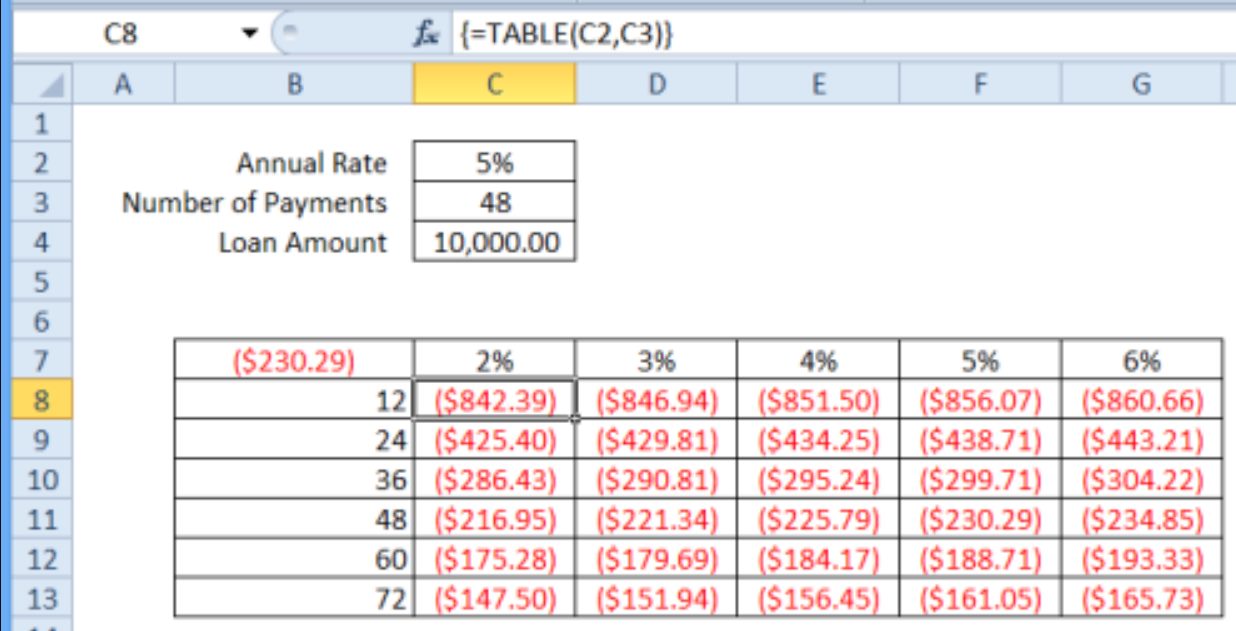
So, grab your mouse and keyboard as we dive into the world of table editing in Excel, sharing tips and tricks that will help you become a data manipulation pro!
Inside This Article
Sorting Data
One of the essential tasks when working with data tables in Excel is sorting the data. Sorting data allows you to organize the information in a specific order, making it easier to analyze and find the desired values. Excel offers a variety of options for sorting data, and it can be done in just a few simple steps.
To sort data in Excel, start by selecting the range of cells that you want to sort. You can choose to sort a single column or multiple columns together. Once you have selected the range, go to the “Data” tab in the Excel ribbon and click on the “Sort” button.
When the Sort dialog box appears, you have the option to sort by one or more columns. You can select the column you want to sort by, choose whether to sort in ascending or descending order, and even add additional sorting levels to further refine your sorting criteria.
Excel also provides the option to sort data based on custom criteria. For example, you can sort data alphabetically, numerically, or by dates. Additionally, you can sort by cell color, font color, or even by using custom formulas.
Once you have defined your sorting criteria, click the “OK” button, and Excel will rearrange the data accordingly. The sorted data will now appear in the order you specified, making it easier to analyze and work with.
Sorting data in Excel is not a permanent action. It rearranges the data temporarily, and you can undo the sorting at any time. This flexibility allows you to experiment with different sorting configurations and revert back to the original order when needed.
Filtering Data
When working with a large dataset in Excel, it can be time-consuming and tedious to scroll through hundreds or even thousands of rows to find specific information. Luckily, Excel provides a powerful feature called “filtering” that allows you to quickly narrow down your data and only display the information you need.
To apply a filter to your data table, start by selecting the entire range of your table. This can be done by clicking and dragging over the data, or by pressing Ctrl+A to select the entire worksheet. Once the data is selected, go to the “Data” tab in the Excel ribbon and click on the “Filter” button.
Once the filter is applied, you will notice small drop-down arrows appear in the header of each column. Clicking on these arrows will reveal a list of unique values in that column. You can then select specific values to filter your data accordingly.
For example, let’s say you have a dataset of sales transactions, and you want to filter the data to only show transactions made by a specific salesperson. You would click on the drop-down arrow in the “Salesperson” column, select the desired salesperson from the list, and Excel will automatically filter the data to show only their transactions.
In addition to filtering by specific values, Excel also allows you to apply advanced filters using criteria. This can be useful when you want to filter data based on multiple conditions or specific ranges. To apply an advanced filter, click on the drop-down arrow in the column you want to filter and select “Filter by Color,” “Filter by Conditional Formatting,” or “Custom Filter” depending on your needs.
Once you have applied the desired filters to your data, you can easily remove them by clicking on the “Filter” button again or by selecting the “Clear Filter” option from the drop-down arrow in any column.
Filtering data in Excel is a powerful way to quickly analyze and manipulate large datasets. Whether you need to find specific information, narrow down options, or perform complex filtering based on criteria, Excel’s filtering feature provides a user-friendly and efficient solution.
Adding or Removing Rows and Columns
When working with data tables in Excel, there may be times when you need to add or remove rows and columns to accommodate new information or to reorganize your data. Excel provides several simple and efficient methods to accomplish this task.
To add a new row, you can right-click on the row number where you want the new row to be inserted, and then select “Insert” from the context menu. Alternatively, you can use the keyboard shortcut Ctrl + Shift + “+”. Excel will insert a new row above the selected row, shifting the existing data downwards.
Similarly, adding a new column can be done by right-clicking on the column letter and choosing “Insert” from the context menu. Alternatively, you can use the keyboard shortcut Ctrl + Shift + “+”. Excel will insert a new column to the left of the selected column, shifting the existing data to the right.
If you need to remove a row, simply select the entire row by clicking on the row number, right-click, and choose “Delete” from the context menu. You can also use the keyboard shortcut Ctrl + “-” to remove the selected row. Be cautious, as this action permanently deletes the row and any associated data.
To remove a column, select the entire column by clicking on the column letter, right-click, and choose “Delete” from the context menu. You can also use the keyboard shortcut Ctrl + “-” to delete the selected column. Again, exercise caution as this action permanently removes the column and any data it contained.
Note that when you add or remove rows or columns, the formulas and formatting in your data table may need adjustment to accommodate the changes. Excel will automatically adjust relative cell references, but it’s essential to review and make any necessary updates to ensure the integrity of your data.
By utilizing the straightforward methods provided by Excel, you can easily add or remove rows and columns in your data tables, allowing you to keep your information organized and up to date.
Overall, editing data tables in Excel is a crucial skill that can greatly enhance your data management capabilities. Whether you need to correct errors, add new information, or organize your data for better analysis, Excel provides a user-friendly interface and a wide range of tools to make the editing process efficient and effective.
By following the step-by-step instructions and utilizing the various techniques discussed in this article, you can confidently manipulate your data tables to meet your specific needs. Remember to always save a backup copy of your original data and make use of Excel’s features like formulas, filters, and sorting options to streamline your editing tasks.
With practice and exploration, you’ll soon become adept at editing data tables in Excel, allowing you to harness the power of your data and make informed decisions. So go ahead, unleash your creativity, and unlock the full potential of your data using Excel’s editing capabilities!
FAQs
Q: How do I edit a data table in Excel?
A: To edit a data table in Excel, follow these steps:
1. Open the Excel file that contains the data table.
2. Click on the cell you want to edit within the data table.
3. Make the necessary changes to the data in the cell.
4. Press Enter or move to another cell to apply the changes.
5. Repeat the process for any other cells you wish to edit in the data table.
Q: Can I edit multiple cells in an Excel data table at once?
A: Yes, you can edit multiple cells in an Excel data table simultaneously by selecting the range of cells you want to edit. To do this, follow these steps:
1. Click and hold on the first cell you want to edit in the data table.
2. Drag your cursor to select the desired range of cells.
3. Make the necessary changes to any of the selected cells.
4. Press Enter or move to another cell to apply the changes to all selected cells simultaneously.
Q: How can I add or remove columns in an Excel data table?
A: To add or remove columns in an Excel data table, follow these steps:
To add a column:
1. Right-click on the column header next to where you want to insert the new column.
2. Click on “Insert” in the context menu.
3. A new column will be added to the left of the selected column.
To remove a column:
1. Click on the column header of the column you want to remove.
2. Right-click on the column header and select “Delete” from the context menu.
3. The selected column and its data will be deleted from the data table.
Q: How can I sort the data in an Excel data table?
A: To sort the data in an Excel data table, follow these steps:
1. Select the entire data table by clicking on any cell within the table.
2. In the Excel toolbar, click on the “Sort & Filter” button.
3. Choose the sorting option you want, such as sorting by a specific column in ascending or descending order.
4. The data table will be sorted according to your selected criteria.
Q: Can I filter data in an Excel data table?
A: Yes, you can filter data in an Excel data table to display only the specific records you want. Here’s how to do it:
1. Select the entire data table by clicking on any cell within the table.
2. Go to the Excel toolbar and click on the “Filter” button.
3. Small arrow icons will appear next to the column headers in the data table.
4. Click on the arrow icon for the column you want to filter.
5. Select the filter criteria you want to apply, such as specific values or text.
6. The data table will be filtered, showing only the records that meet your selected criteria.