
Are you looking to import a data set into R for analysis and modeling? Look no further, as this comprehensive guide will walk you through the process step by step. R is a powerful programming language commonly used for statistical analysis and data visualization. With its vast array of libraries and packages, it offers a wide range of tools for handling and manipulating data sets. Whether you are a beginner or an experienced data scientist, understanding how to import data into R is a fundamental skill that will set you on the path to successful data analysis. In this article, we will explore different methods of importing data into R, including reading data from CSV files, Excel spreadsheets, databases, and web APIs. So, let’s dive in and learn how to import data sets into R!
Inside This Article
- Installing the Necessary Packages
- Loading the Dataset
- Understanding the Data Structure
- Handling Missing Data
- Exploring the Dataset
- Conclusion
- FAQs
Installing the Necessary Packages
Before we can import a data set into R, we need to make sure we have the necessary packages installed. These packages contain functions and tools that allow us to work with the data effectively. Thankfully, installing packages in R is straightforward and can be done in a few simple steps.
To begin, open your R console or RStudio. Then, use the following syntax to install a package:
install.packages("package_name")
Replace “package_name” with the name of the specific package you need. For example, if you want to install the popular “tidyverse” package, the command would be:
install.packages("tidyverse")
Once you’ve entered the command, hit enter, and R will start downloading the package from the appropriate repository. This may take a few moments, depending on your internet connection speed.
After the package is installed, you only need to install it once. From that point forward, you can load the package into your R session whenever you need to use it.
To load a package, use the following syntax:
library(package_name)
Again, replace “package_name” with the name of the package you want to load. For example, if you want to load the “tidyverse” package, the command would be:
library(tidyverse)
Now you’re ready to import your data set into R and start analyzing it! By installing the necessary packages, you gain access to powerful tools that make data manipulation and visualization much easier. Make sure to explore the documentation for each package to fully utilize its capabilities and take your data analysis to the next level.
Loading the Dataset
Once you have installed the necessary packages for R, you are ready to load your dataset. Loading the dataset is a crucial step in any data analysis or machine learning project, as it allows you to access and manipulate the data for further analysis.
In R, there are multiple ways to load a dataset, depending on the format in which the data is stored. Let’s explore some of the common methods for loading datasets:
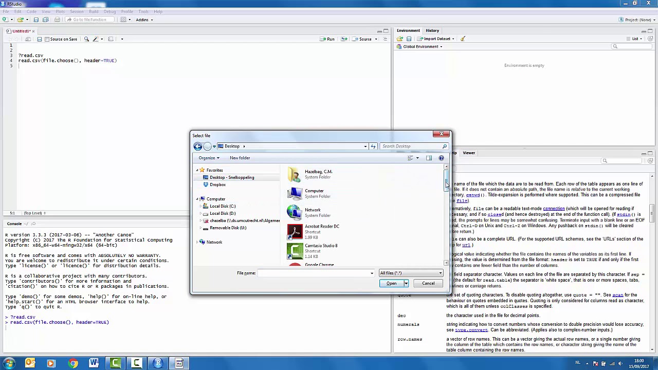
- Using read.csv(): If the dataset is stored in a CSV (Comma Separated Values) file, you can use the
read.csv()function to load it. This function reads the CSV file and returns a data frame, which is a common data structure in R for storing tabular data. - Using read.table(): If the dataset is not in CSV format, but rather in a plain text file with a specific delimiter (such as tab or semicolon), you can use the
read.table()function. This function allows you to specify the delimiter and other parameters to correctly read the data from the file. - Using read_excel(): If the dataset is in an Excel file format (xls or xlsx), you can use the
read_excel()function from the “readxl” package to load the data into R. This function provides convenient options for reading specific sheets or ranges of data from Excel files. - Using readRDS(): R also allows you to save and load datasets in its own binary format using the
saveRDS()andreadRDS()functions. This can be useful when you want to preserve the entire structure of the dataset, including any custom attributes or metadata.
It is important to note that the specific function and parameters to use for loading your dataset will depend on the file format and characteristics of your data. For more detailed information on each loading method, you can refer to the documentation of the respective functions in R.
Once the dataset is successfully loaded, you can verify this by using R’s built-in functions to examine the structure and preview the data. This will allow you to ensure that the dataset has been loaded correctly and to perform any necessary data cleaning or preprocessing steps before proceeding with your analysis.
Understanding the Data Structure
When working with data in R, it is crucial to have a clear understanding of the structure of the dataset. This includes knowing the number of variables, the types of variables, and how the data is organized.
R provides various functions that can help you gain insights into the structure of your dataset. One such function is the str() function, which stands for “structure”. It displays a concise and informative summary of the data, including the number of observations, the number of variables, and the data type of each variable.
For example, let’s say you have imported a dataset into R and assigned it to a variable called my_data. To understand its structure, you can simply call str(my_data):
str(my_data)
The output of this command will provide you with valuable information such as the number of observations, variables, and the type of each variable. This can be particularly helpful when dealing with large datasets or when you need to quickly glance at the overall structure of the data.
In addition to the str() function, you can also use the summary() function to obtain summary statistics for each variable in your dataset. This function provides measures such as minimum, maximum, mean, median, and quartiles.
By understanding the structure of your data, you can make informed decisions on how to manipulate and analyze it. For example, if you have a categorical variable, you may need to convert it into a factor. On the other hand, if you have missing values, you may need to handle them using techniques such as imputation or deletion.
Moreover, understanding the data structure allows you to identify potential data quality issues. For instance, if you notice that a numerical variable is being treated as a character variable, you can take the necessary steps to convert it into the correct data type.
Overall, gaining a comprehensive understanding of the data structure is an essential step in any data analysis project. It aids in data cleaning, variable transformation, and accurate interpretation of results.
Handling Missing Data
Dealing with missing data is a critical step in data analysis. Missing values can significantly impact the accuracy and reliability of your analysis results. Fortunately, R provides various techniques to handle missing data effectively.
One common approach to handling missing data is to remove any rows or columns with missing values. This method, known as complete case analysis or listwise deletion, is straightforward but may lead to a loss of valuable information if the missing values are randomly distributed across the dataset.
R offers the na.omit() function, which can be used to remove rows with missing values. For example:
data <- na.omit(data)
If you have a large dataset, removing missing data may not be a viable option. In such cases, imputation techniques can be used to estimate and fill in the missing values.
One popular imputation method is mean imputation, where missing values are replaced with the mean of the corresponding variable. R provides the na.mean() function from the impute package for mean imputation. Here's an example:
library(impute)

data$column <- na.mean(data$column)
Another common imputation method is regression imputation, where missing values are predicted based on the values of other variables using a regression model. The mice package in R provides comprehensive tools for regression imputation. Here's how you can perform regression imputation:
library(mice)

imputed_data <- mice(data)
completed_data <- complete(imputed_data)
In addition to these methods, R also provides other advanced imputation techniques, such as k-nearest neighbors imputation and multiple imputations. These techniques are especially useful when dealing with complex datasets.
It is important to note that the choice of imputation method should depend on the nature of the data and the specific analysis goals. You should also consider the potential biases that imputation may introduce into your dataset.
Before applying any imputation method, it is essential to thoroughly understand the pattern and nature of missing data. Visualizations, such as bar charts or heatmaps, can help identify any patterns or correlations between missing values and other variables. This understanding can guide your choice of the most appropriate imputation technique.
Overall, handling missing data in R requires a combination of careful analysis, knowledge of imputation methods, and consideration of the specific dataset and analysis goals. By implementing appropriate techniques, you can minimize the impact of missing data on your analysis results and ensure the integrity of your findings.
Exploring the Dataset
Now that we have successfully loaded the dataset into R, it's time to dive into the exciting task of exploring and understanding the data. Exploring the dataset is a crucial step in any data analysis process as it helps to uncover patterns, trends, and insights that can drive decision-making.
Let's start by obtaining a summary of the dataset. In R, we can use the summary() function to get a quick overview of the variables in the dataset. This function provides important information such as the minimum and maximum values, mean, median, and quartiles for each variable. It also identifies any missing values in the dataset, giving us an idea of the data quality.
After obtaining the summary, it's time to take a closer look at each variable individually. We can use various functions in R to gain insights into different aspects of the dataset. For numerical variables, we can calculate measures of central tendency (mean, median) and dispersion (standard deviation, range) to understand the distribution and variation. Visualizing the data using histograms, box plots, or scatter plots can also provide a visual representation of the distribution and any outliers.
For categorical variables, we can use frequency tables to observe the distribution of different categories. Bar plots or pie charts can be used to visualize the proportions of each category. This helps us understand the prevalence of different categories and identify any patterns or imbalances.
In addition to exploring individual variables, it's important to explore the relationships between variables. By calculating correlation coefficients, we can determine the strength and direction of relationships between numerical variables. Scatter plots or heatmaps can visually represent these relationships. For categorical variables, cross-tabulation or stacked bar plots can be used to identify associations.
As we explore the dataset, it's important to keep an eye out for any inconsistencies or outliers. These could be in the form of missing values, extreme values, or unexpected patterns. It's essential to handle these outliers appropriately, either by removing them, imputing missing values, or transforming the data if necessary.
Exploring the dataset also involves looking for specific patterns, trends, or anomalies that are relevant to the analysis. This could include seasonality in time series data, sudden spikes or drops in a variable, or unusual patterns that warrant further investigation. By being thorough in our exploration, we can gain a deeper understanding of the dataset and make informed decisions in our analysis.
Remember, exploring the dataset is not a one-time task. It is an iterative process that can involve revisiting and updating our analysis as new insights are gained. By continuously exploring the dataset, we can uncover hidden patterns and uncover valuable insights that can drive actionable outcomes.
Conclusion
Importing a data set into R is a fundamental skill for data analysts and scientists. With the various methods and packages available, such as read.csv(), read.table(), and read_excel(), you have the flexibility to import data from different file formats.
In this article, we have covered how to import data sets into R using these methods. We have explored the different options to specify file paths, set delimiter options, and handle missing values. Additionally, we have discussed the benefits of using tidyverse packages like readr and haven for more efficient and streamlined data importing.
Remember to keep in mind the best practices when importing data sets, including understanding the structure of your data, handling errors and missing values, and properly documenting your workflow. With these techniques and approaches, you can confidently import and analyze data in R, unlocking valuable insights for your research or business needs.
So, whether you are working with CSV, TXT, or Excel files, you now have the knowledge and tools to seamlessly import your data sets into R and embark on your data analytics journey.
FAQs
1. Can I import data sets from different file formats into R?
Absolutely! R supports importing data from various file formats such as CSV, Excel, SPSS, SAS, and more. It provides specific packages and functions to handle each file format, making it versatile and flexible for data analysts.
2. What is the most common way to import a CSV file into R?
The most common way to import a CSV file into R is by using the "read.csv()" function. This function reads the data from a CSV file and creates a data frame in R, which is a common structure for storing and working with data.
3. How can I import an Excel file into R?
To import an Excel file into R, you can use the "read_excel()" function from the "readxl" package. This function allows you to read data from both .xls and .xlsx files and create a data frame in R.
4. Is it possible to import data sets from online sources directly into R?
Yes, it is possible to import data sets from online sources directly into R. There are packages such as "readr" and "httr" that can be used to download data from URLs and read it into R. This is particularly useful when working with live, updated data sets.
5. Can I import data sets from databases into R?
Definitely! R provides packages like "DBI" and "RMySQL" that allow you to connect to databases such as MySQL, PostgreSQL, and SQLite and import data directly into R. This enables seamless analysis and manipulation of large-scale datasets stored in databases.