
Matching data from two Excel sheets can be a common task when working with spreadsheets. Whether you’re comparing sales figures from different periods, cross-referencing customer information, or consolidating data from multiple sources, knowing how to match data accurately can save you time and effort.
Excel provides several built-in functions and techniques to help you match data across multiple sheets. From using VLOOKUP or INDEX/MATCH formulas to conditional formatting and sorting, there are various approaches you can take based on your specific requirements.
In this article, we will explore different methods to match data from two Excel sheets, including step-by-step instructions and tips to ensure accurate results. Whether you’re a beginner or an experienced Excel user, by the end of this article, you’ll have a solid understanding of how to effectively match data from two Excel sheets.
Inside This Article
- Overview
- Method 1: VLOOKUP Function
- Method 2: INDEX and MATCH Functions
- Method 3: Using Power Query
- Conclusion
- FAQs
Overview
Matching data from two Excel sheets is a common task that often arises when working with large datasets. It involves finding matching values in one sheet and retrieving corresponding data from another sheet. This can be a time-consuming and tedious process, especially when dealing with a large number of records. Luckily, there are several methods available in Excel that make this task much easier and more efficient.
In this article, we will explore three popular methods for matching data from two Excel sheets:
- VLOOKUP Function: The VLOOKUP function is a powerful tool in Excel that allows you to search for a value in one column and retrieve a corresponding value from another column. This method is straightforward and suitable for basic matching tasks.
- INDEX and MATCH Functions: The combination of the INDEX and MATCH functions provides more flexibility and control compared to VLOOKUP. It allows you to search for a value in one column and retrieve data from any column in the same row. This method is particularly useful when dealing with complex data structures.
- Using Power Query: Power Query is a powerful data transformation and manipulation tool in Excel. It allows you to connect to multiple data sources, merge tables, and perform complex transformations. This method is perfect for handling large datasets and automating the matching process.
By exploring these different methods, you’ll gain a deeper understanding of how to efficiently match data from two Excel sheets, regardless of the complexity of your data. So let’s dive in and discover the power of Excel in matching and retrieving data!
Method 1: VLOOKUP Function
The VLOOKUP function is a powerful tool in Excel that allows you to search for a value in one column of data and retrieve a corresponding value from another column. It is particularly handy when you need to match data from two different Excel sheets. Here’s how you can use the VLOOKUP function to accomplish this:
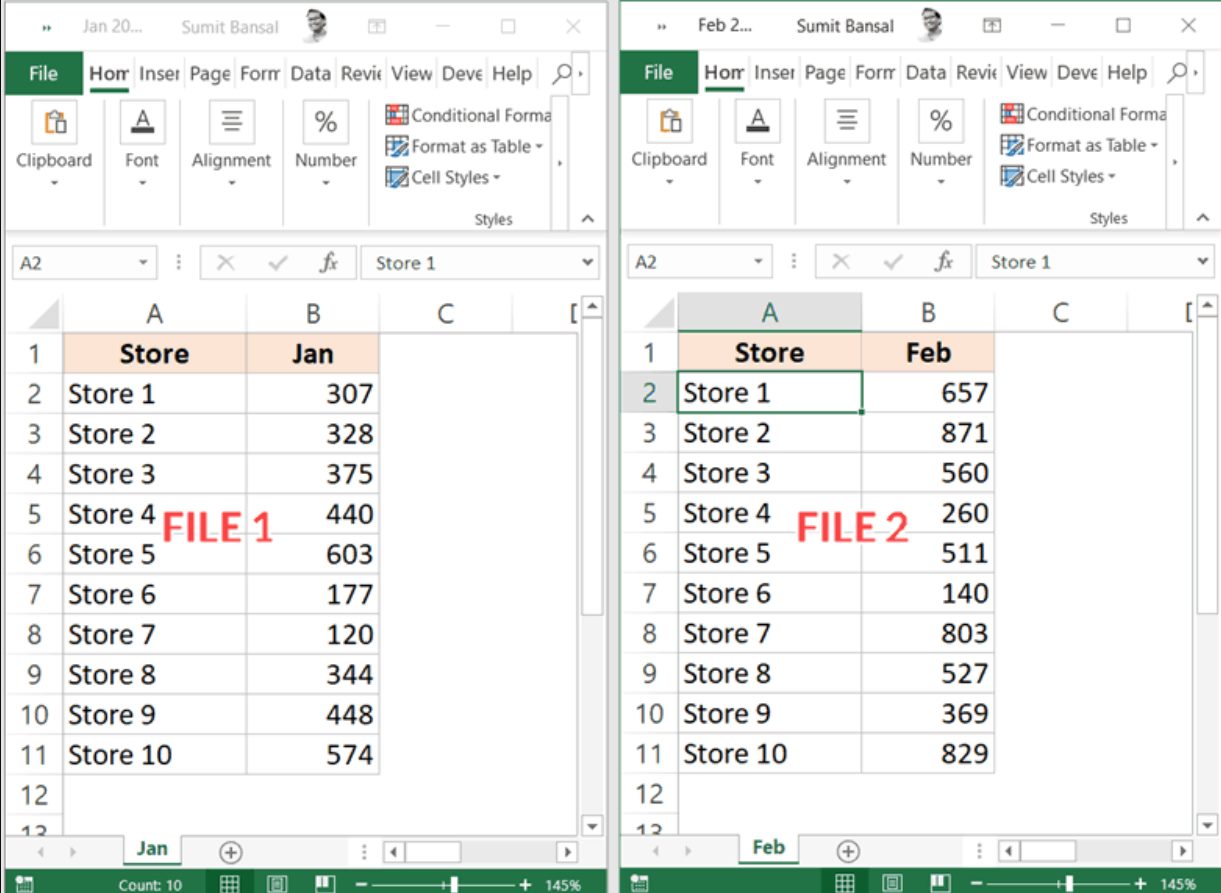
Step 1: First, open both Excel sheets that contain the data you want to match. Make sure that both sheets have a common key or unique identifier that you can use to connect the data.
Step 2: In the sheet where you want to retrieve the data, select a cell where you want the matched data to appear. This is where you will write the VLOOKUP formula.
Step 3: Begin writing the VLOOKUP formula by typing “=VLOOKUP(“. This will prompt Excel to guide you through the syntax of the function.
Step 4: Now, you need to specify three main arguments for the VLOOKUP function:
- The lookup value: This is the value you want to search for in the first column of the other sheet.
- The table array: This is the range of cells that contains the data you want to match, including both the lookup column and the desired result column.
- The column index number: This is the column number (counting from the left) in the table array that contains the desired result.
Step 5: Fill in the arguments for the VLOOKUP function. For example, if your lookup value is in cell A2, the table array is in Sheet2!A:B, and the desired result is in the second column, your VLOOKUP formula would look like this:
=VLOOKUP(A2, Sheet2!A:B, 2, FALSE)
Step 6: Press Enter to apply the VLOOKUP formula. Excel will now search for the lookup value in the specified range and return the corresponding value from the desired column.
Step 7: Copy the formula down to the rest of the cells in the column to match the data for all the rows in your sheet.
The VLOOKUP function provides a quick and effective way to match data from two Excel sheets. It is essential to understand the arguments and syntax of the function to maximize its usefulness. With practice, you will be able to match data effortlessly and save valuable time and effort in your data analysis tasks.
Method 2: INDEX and MATCH Functions
When it comes to matching data from two Excel sheets, another powerful method is to use the combination of the INDEX and MATCH functions. This method allows you to look up a value in one sheet based on matching criteria in another sheet.
The INDEX function is used to retrieve a value from a specific row and column in a specified range. The MATCH function, on the other hand, is used to find the position of a specified value within a range. By using these two functions together, you can locate and extract the desired data from two different sheets.
Here are the steps to use the INDEX and MATCH functions for matching data:
- In your destination sheet, select the cell where you want to display the matched data.
- Enter the following formula:
=INDEX([Range],MATCH([Lookup Value],[Lookup Range],0)) - Replace
[Range]with the range where the desired data is located in the source sheet. - Replace
[Lookup Value]with the value you want to match. - Replace
[Lookup Range]with the range where the matching criteria are located in the source sheet. - Press Enter to apply the formula and retrieve the matched data.
By using the INDEX and MATCH functions, you can perform advanced data matching and retrieval in Excel. This method gives you more flexibility and control over the matching process, allowing you to customize the search criteria and handle complex matching scenarios.
It is worth noting that the INDEX and MATCH functions are not limited to matching data between two sheets. You can use them to match data within the same sheet or even across multiple workbooks, making them versatile tools for data analysis and manipulation.
Overall, the INDEX and MATCH functions provide a robust and efficient method for matching data in Excel. They offer flexibility, accuracy, and the ability to handle complex matching scenarios. Whether you are working with large datasets or need to perform advanced data analysis, leveraging these functions will greatly enhance your Excel skills.
Method 3: Using Power Query
If you’re looking for a powerful and efficient way to match data from two Excel sheets, using Power Query is an excellent option. Power Query allows you to combine, transform, and refine data from multiple sources, making it an ideal tool for matching data in Excel.
Here’s a step-by-step guide on how to use Power Query to match data from two Excel sheets:
- Open Excel and navigate to the Data tab.
- Click on the “Get Data” button and select “Combine Queries” from the drop-down menu.
- In the Combine Queries dialog box, choose “Append” as the option to merge the two queries.
- Select the first sheet you want to match data from and click “OK”.
- Repeat step 4 for the second sheet.
- In the Power Query Editor, select the columns you want to match data on.
- Right-click on one of the selected columns and choose “Merge” from the context menu.
- In the Merge dialog box, select the second sheet as the “Right” table and choose the desired matching options.
- Click “OK” to merge the two queries and create a new table with the matched data.
- Close the Power Query Editor and load the resultant table into Excel.
Using Power Query not only allows you to match data from two Excel sheets but also provides additional capabilities such as filtering, sorting, and transforming data. It’s a versatile tool that helps streamline data analysis and manipulation tasks.
Keep in mind that Power Query is available in newer versions of Excel, such as Excel 2010 onwards. So, make sure you have the appropriate version to access this powerful feature.
By following these steps, you can effectively match data from two Excel sheets using Power Query. Experiment with different matching options and explore the various functionalities offered by Power Query to enhance your data analysis capabilities.
Conclusion
In conclusion, matching data from two Excel sheets can be a complex process, but with the right techniques and tools, it becomes much more manageable. By utilizing functions like Vlookup, Index Match, and Power Query, you can easily compare and merge data from multiple sheets. These methods help ensure accuracy and efficiency in your data analysis tasks.
Furthermore, investing time into understanding the nuances of Excel formulas, sorting, and filtering can greatly improve your ability to match data effectively. Don’t be afraid to experiment and explore different approaches to find the one that works best for your specific situation.
Remember, practice makes perfect. The more you work with Excel and understand its functionality, the more comfortable you will become with matching data from different sheets. So, embrace the process, hone your skills, and soon you’ll excel in Excel!
FAQs
Q: How do I match data from two Excel sheets?
A: To match data from two Excel sheets, you can use the VLOOKUP function. This function allows you to search for a value in one sheet and retrieve matching data from another sheet based on a common identifier. Simply enter the VLOOKUP formula in the target sheet and specify the lookup value, the range to search in, the column index for the desired data, and the match type.
Q: Can I match data from two sheets without using a formula?
A: Yes, you can match data from two Excel sheets without using a formula. One way is to use the “Copy and Paste” method. You can copy the data from one sheet and paste it into another, aligning the common identifiers in both sheets. Another option is to use the “Match Destination Formatting” paste option, which matches the formatting of the destination sheet while pasting the data.
Q: Can I match data from two sheets with different column names?
A: Yes, you can match data from two sheets with different column names. In such cases, you will need to use a combination of functions like INDEX and MATCH. The MATCH function helps find the position of the common identifier in both sheets, and then the INDEX function retrieves the corresponding data based on the matched position.
Q: How can I quickly identify unmatched data between two Excel sheets?
A: You can quickly identify unmatched data between two Excel sheets by using the VLOOKUP or INDEX-MATCH functions. By checking for errors or #N/A values in the result column, you can easily identify the data that does not have a match in the other sheet.
Q: Is there a way to automate the matching of data between multiple Excel sheets?
A: Yes, you can automate the matching of data between multiple Excel sheets using macros or VBA (Visual Basic for Applications). By writing custom code, you can create a script that searches, matches, and retrieves data from multiple sheets automatically, saving time and effort.