How To Match Data In Two Excel Sheets Using Vlookup

If you’re looking to match data in two separate Excel sheets, then you’re in the right place. One of the most commonly used functions for this purpose is Vlookup, which allows you to search for a specific value in one sheet and retrieve corresponding information from another sheet.

Whether you’re trying to consolidate data from different sources or simply cross-reference information, Vlookup can be a powerful tool to help you save time and effort. In this article, we’ll take you through the steps of using Vlookup to match data in two Excel sheets.

By the end of this guide, you’ll have a clear understanding of how to utilize Vlookup effectively and efficiently in your Excel spreadsheets. So, let’s dive into the world of data matching and start harnessing the full potential of Vlookup!

Inside This Article

1. Overview of Vlookup Function
2. Step 1: Open the Excel Sheets
3. Step 2: Identify the Matching Column
4. Step 3: Use Vlookup Function to Match Data
5. Conclusion
6. FAQs

Overview of Vlookup Function

The Vlookup function is one of the most powerful and commonly used functions in Microsoft Excel. It allows you to find and retrieve specific information from a large dataset by searching for a value in one column and returning the corresponding value from another column. Vlookup stands for “vertical lookup,” which means it looks for the value in a vertical column and retrieves information from the same row.

By using Vlookup, you can easily match data between two different Excel sheets based on a common identifier or key. This function is particularly useful when dealing with large datasets or when you need to consolidate information from multiple sources.

The Vlookup function takes four arguments: the value you want to search for, the table array that contains the data, the column index number for the value you want to retrieve, and an optional range lookup value that specifies whether you want an exact match or an approximate match. When using Vlookup to match data in two Excel sheets, you need to carefully select the appropriate arguments to ensure accurate results.

Overall, the Vlookup function is a powerful tool that can save you significant time and effort when working with large datasets. Understanding how to use Vlookup to match data in Excel sheets is a valuable skill that can help you manipulate and analyze data more efficiently.

Step 1: Open the Excel Sheets

Before we can start matching the data in two Excel sheets using the Vlookup function, the first step is to open the Excel sheets that contain the data you want to compare. It is essential to have both sheets accessible in order to proceed with the matching process.

To open an Excel sheet, simply navigate to the location where the file is saved and double-click on it. This will launch the Microsoft Excel application and open the sheet in a new window.

If you have multiple Excel sheets that need to be matched, it is recommended to open them in separate windows or tabs. This will enable you to easily reference and switch between the sheets as you perform the Vlookup function.

It is also important to ensure that both Excel sheets are formatted correctly for the matching process. Make sure that the data you want to compare is organized in separate columns and rows. This will help streamline the matching process and ensure accurate results.

Once you have opened the Excel sheets and ensured that the data is properly organized, you are now ready to move on to the next step: identifying the matching columns.

Step 2: Identify the Matching Column

In order to match data between two Excel sheets using Vlookup, you need to first identify the column that contains the common key or identifier. This key will be used to search for matching values in the second Excel sheet.

Here are the steps to follow:

1. Open both Excel sheets: Start by opening the two Excel sheets that you want to compare and match the data between. Make sure you have the necessary permissions to access and modify these sheets.
2. Identify the common key column: Look for a column that exists in both sheets and contains unique values that can be used as the basis for matching. This column could be a unique identifier like an ID number or a common attribute like a name or date. It’s important that this column is present in both sheets and has the same type of data.
3. Make note of the column header: Once you have identified the common key column, take note of its column header. This will help you properly reference the column in the Vlookup formula.
4. Ensure data consistency: Check that both sheets have consistent data in terms of formatting, data types, and spelling. Any discrepancies or inconsistencies in the data may lead to inaccuracies or failed matches.

It is important to properly identify the matching column upfront to ensure accurate data matching between the two Excel sheets. Taking the time to carefully select and verify the common key column will enhance the success of using Vlookup to match the data.

Step 3: Use Vlookup Function to Match Data

Now that you have identified the matching column in both Excel sheets, it’s time to utilize the powerful Vlookup function to match the data. The Vlookup function is a built-in Excel function that allows you to search for a value in one column and retrieve the corresponding value from another column in the same row.

To use the Vlookup function, follow these steps:

1. Click on an empty cell in the sheet where you want to display the matching data.
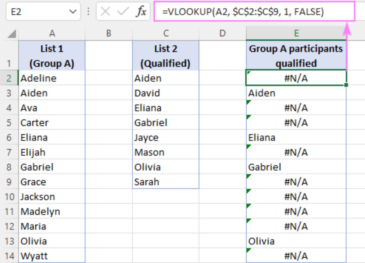
2. Type the Vlookup formula: =VLOOKUP(lookup_value, table_array, col_index_num, [range_lookup])
3. Replace the lookup_value with the cell reference that contains the value you want to match.
4. Replace the table_array with the range that contains the data you want to search in.
5. Replace the col_index_num with the number that represents the column index of the data you want to retrieve.
6. Specify whether you want an exact match or an approximate match by adding range_lookup (optional). Use TRUE for an approximate match and FALSE for an exact match.
7. Press Enter to execute the formula.

Once you have entered the Vlookup formula, Excel will search for the specified value in the table_array and return the corresponding value from the col_index_num.

For example, let’s say you have a list of employee IDs in column A of Sheet 1, and you want to match the employee names from column B of Sheet 2. You can use the Vlookup function to retrieve the employee names based on the matching IDs.

By using the Vlookup function, you can quickly and efficiently match data between two Excel sheets. It eliminates the need for manual searching and saves you time and effort. Plus, it ensures accuracy and consistency in your data matching process.

Remember, the Vlookup function may return an error if it fails to find the matching value. In such cases, you can use the IFERROR function to handle the error gracefully and display a custom message or value.

With the Vlookup function, you have a powerful tool at your disposal to easily match data between two Excel sheets. Use this function to streamline your data analysis and make informed decisions based on accurate and up-to-date information.

Conclusion

Matching data in two Excel sheets can be a valuable tool for analyzing and comparing information. The VLOOKUP function provides a powerful and flexible way to accomplish this task. By following the steps outlined in this article, you can easily match data between two Excel sheets and gain deeper insights into your data.

Remember, a successful matching process requires careful selection and understanding of the key columns, as well as ensuring the data formats are compatible. Additionally, organizing your data in a consistent and standardized manner will greatly facilitate the matching process.

Whether you are a business professional, researcher, or student, being able to match data in Excel can save you time and effort in your data analysis tasks. By mastering the VLOOKUP function, you will have a powerful tool at your disposal to efficiently compare and combine data across multiple datasets.

FAQs

1. What is Vlookup?
Vlookup is a powerful function in Excel that allows you to search for a specific value in a table or range and return a corresponding value from another column in that table. It is commonly used to match data between two different Excel sheets.

2. How does Vlookup work?
Vlookup works by searching for a value in the first column of a specified range and returning the corresponding value from a specific column within that range. It uses the following syntax: VLOOKUP(lookup_value, table_array, col_index_num, range_lookup).

3. Can Vlookup be used to match data in two different Excel sheets?
Yes, Vlookup can be used to match data in two different Excel sheets. By using the extended syntax of the Vlookup function, you can specify a table array that includes a range from another sheet.

4. How do I use Vlookup to match data in two Excel sheets?
To use Vlookup to match data between two Excel sheets, follow these steps:
– In the first sheet, identify the column that contains the value you want to match.
– In the second sheet, identify the column that contains the matching values.
– In the second sheet, use the Vlookup function to search for the matching values in the first sheet and return the desired data.

5. Are there any limitations to using Vlookup to match data in two Excel sheets?
Yes, there are some limitations to using Vlookup to match data in two Excel sheets:
– The data you want to match must be in the leftmost column of the table array.
– Both sheets must have a common column that can be used as a reference for matching.
– Vlookup only returns the first match it finds, so if there are multiple matches, it will only return the first one.