
If you’re an Excel user, you may have come across the frustrating issue of blank cells scattered between your data. These empty cells can make your spreadsheet look cluttered and make it harder to analyze the information effectively. Fortunately, there are ways to remove these blank cells and streamline your data in Excel.
In this article, we will guide you through the process of removing blank cells between data in Excel, helping you clean up your spreadsheet and improve its readability. Whether you’re working with a large dataset or a simple table, we’ll provide you with step-by-step instructions and useful tips to eliminate those pesky blank cells.
So, if you’re ready to organize your data and make your Excel spreadsheet look more professional, let’s dive into the methods for removing blank cells between your data!
Inside This Article
- Method 1: Using Go To Special
- Method 2: Using Filter
- Method 3: Using Formulas
- Method 4: Using VBA Macro
- Conclusion
- FAQs
Method 1: Using Go To Special
Removing blank cells between data in Excel can be easily accomplished using the Go To Special feature. Here’s a step-by-step guide on how to do it:
-
Select the range of cells containing the data and blank cells.
-
Open the Go To Special dialog box. To do this, you can press the shortcut key Ctrl + G or navigate to the Home tab, click on the Find & Select dropdown arrow, and select “Go To Special”.
-
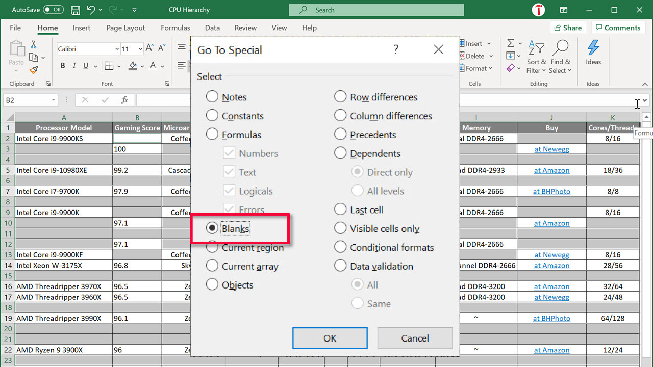
In the Go To Special dialog box, select the “Blanks” option and click on the “OK” button.
-
All the blank cells in the selected range will now be highlighted.
-
Right-click on one of the selected blank cells and choose “Delete” from the context menu.
By following these simple steps, you can quickly remove the blank cells between your data in Excel, making your spreadsheet more organized and easier to work with.
Method 2: Using Filter
Step 1: Select the range of cells containing the data. This can be done by clicking and dragging to highlight the desired range.
Step 2: Click on the ‘Filter’ button located in the Data tab of the Excel toolbar. This will enable the filter functionality for the selected range of cells.
Step 3: Once the filter is enabled, you will notice filter arrows appearing in the column headers. Click on the filter arrow for the column that contains the blank cells.
Step 4: In the filter dropdown menu, uncheck the ‘Blanks’ option. This will filter out all the blank cells from the selected column, leaving only the cells with data visible.
Step 5: With the blank cells filtered out, you can now select all the visible cells in the column (excluding the blank cells). You can do this by clicking on the first cell, holding the Shift key, and clicking on the last visible cell in the column.
Finally, you can delete the selected cells by right-clicking on any of the selected cells and choosing the ‘Delete’ option from the context menu. This will remove the selected cells, including the blank cells, from the worksheet, leaving only the cells with data intact.
Method 3: Using Formulas
One method to remove blank cells between data in Excel is by using formulas. This technique involves using the IF function to identify the blank cells and then replacing them with the desired values.
Step 1: Use the IF function to identify the blank cells in a new column
In this step, you need to create a new column next to the original data. In the first cell of the new column, use the IF function to check if the corresponding cell in the original data is blank. The formula would look like this:
=IF(ISBLANK(A2),"",A2)
Where A2 is the cell reference of the first cell containing the data in the original column. This formula checks if the cell is blank and returns an empty string if it is, otherwise it returns the value in the cell.
Step 2: Copy the formula down to apply it to all the cells in the column
Once you have entered the formula in the first cell of the new column, you need to copy it down to apply it to all the cells in the column. You can simply drag the fill handle (the small square at the bottom-right corner of the selected cell) down to fill the formula in the remaining cells. This will check each corresponding cell in the original column and display the value if it is not blank.
Step 3: Select and copy the column containing the formula results
Next, you need to select the entire column containing the formula results. Click on the header of the new column to select the entire column.
Step 4: Paste the values over the original data, replacing the formulas
Once the column with the formula results is selected, right-click and choose ‘Copy’ from the context menu. Then, select the first cell in the original data column, right-click again, and choose ‘Paste Values’ from the context menu. This will paste the values from the formula column over the original data, replacing the formulas with the actual values.
Step 5: Delete the column with the formula
Now that you have replaced the blank cells with the desired values, you can delete the column with the formula. Simply right-click on the column header of the formula column and choose ‘Delete’ from the context menu. This will remove the column and leave you with a clean dataset without any blank cells.
By following these steps, you can easily remove blank cells between data in Excel using formulas. This method provides a quick and efficient way to clean up your data and ensure accuracy and consistency.
Method 4: Using VBA Macro
Step 1: Press Alt+F11 to open the Visual Basic for Applications (VBA) editor.
Step 2: Insert a new module.
Step 3: Copy and paste the VBA code for removing blank cells.
Step 4: Press F5 to run the macro and remove the blank cells.
VBA macros offer a powerful way to automate tasks in Excel, including the removal of blank cells. By following these simple steps, you can quickly and efficiently remove the blank cells between your data. Here’s how:
Step 1: Press Alt+F11 to open the Visual Basic for Applications (VBA) editor. This will open a new window where you can write and edit VBA code.
Step 2: Insert a new module. In the VBA editor, go to the “Insert” menu and select “Module.” This will create a blank module where you can write your VBA code.
Step 3: Copy and paste the VBA code for removing blank cells. Below is a sample VBA code that you can use:
Sub RemoveBlankCells()

    Dim rng As Range

    Set rng = Selection.SpecialCells(xlCellTypeBlanks)

    rng.Delete Shift:=xlUp

End Sub
This code uses the xlCellTypeBlanks constant to select all the blank cells in the currently selected range and then deletes them by shifting the remaining cells up.
Step 4: Press F5 to run the macro and remove the blank cells. To execute the VBA code, simply press the F5 key or go to the “Run” menu and select “Run Sub/UserForm.” This will run the macro and remove the blank cells in the selected range.
Using VBA macros can save you a significant amount of time and effort when dealing with large datasets in Excel. It provides a flexible and customizable solution to remove blank cells between your data.
Remember, before running any VBA macro, it is always a good practice to save your work and create a backup copy of your Excel file, as macros can modify data. Additionally, make sure to test the macro on a small subset of your data to ensure the desired results before running it on the entire dataset.
By following these steps, you can utilize VBA macros to remove blank cells in Excel, streamlining your data organization and improving your workflow.
Conclusion
In conclusion, knowing how to remove blank cells between data in Excel can greatly enhance your productivity and improve the accuracy and efficiency of your spreadsheet. Whether you are dealing with a large dataset or simply want to tidy up your data, the techniques outlined in this article can help you achieve your goals.
By using the filters, functions, and formatting options available in Excel, you can easily identify and remove any unnecessary blank cells that may be impacting your analysis or calculations. Additionally, the use of formulas and macros can automate the process, saving you time and effort.
Remember to always make a backup of your data before making any changes, and familiarize yourself with the different techniques to ensure you choose the most suitable method for your specific needs. With these strategies in your toolkit, you’ll be able to clean up your spreadsheets and work with cleaner, more reliable data in no time.
FAQs
Q: How can I remove blank cells between data in Excel?
Removing blank cells between data in Excel can be done by following these steps:
1. Select the range of cells where you want to remove the blank cells.
2. Press `Ctrl+G` or click on the “Go To” dialog box launcher in the ribbon’s “Editing” group.
3. In the “Go To” dialog box, click on the “Special” button.
4. In the “Go To Special” dialog box, select the “Blanks” option and click “OK”.
5. Right-click on any of the selected blank cells and choose “Delete” from the context menu.
6. In the “Delete” dialog box, select the “Shift cells up” option and click “OK”.
7. The blank cells between the data will be removed.
Q: Is there any way to remove blank cells without affecting the surrounding data?
Yes, there is a way to remove blank cells without affecting the surrounding data. Follow these steps:
1. Select the range of cells where you want to remove the blank cells.
2. Press `Ctrl+G` or click on the “Go To” dialog box launcher in the ribbon’s “Editing” group.
3. In the “Go To” dialog box, click on the “Special” button.
4. In the “Go To Special” dialog box, select the “Blanks” option and click “OK”.
5. Right-click on any of the selected blank cells and choose “Delete” from the context menu.
6. In the “Delete” dialog box, select the “Entire row” option and click “OK”.
7. The blank cells will be removed without affecting the surrounding data.
Q: Is it possible to remove blank cells in a specific column?
Yes, you can remove blank cells in a specific column by following these steps:
1. Select the column where you want to remove the blank cells.
2. Press `Ctrl+G` or click on the “Go To” dialog box launcher in the ribbon’s “Editing” group.
3. In the “Go To” dialog box, click on the “Special” button.
4. In the “Go To Special” dialog box, select the “Blanks” option and click “OK”.
5. Right-click on any of the selected blank cells and choose “Delete” from the context menu.
6. In the “Delete” dialog box, select the “Shift cells up” option and click “OK”.
7. The blank cells in the specific column will be removed.
Q: How can I remove blank cells in a row?
To remove blank cells in a row, follow these steps:
1. Select the row where you want to remove the blank cells.
2. Press `Ctrl+G` or click on the “Go To” dialog box launcher in the ribbon’s “Editing” group.
3. In the “Go To” dialog box, click on the “Special” button.
4. In the “Go To Special” dialog box, select the “Blanks” option and click “OK”.
5. Right-click on any of the selected blank cells and choose “Delete” from the context menu.
6. In the “Delete” dialog box, select the “Shift cells left” or “Shift cells right” option based on your preference and click “OK”.
7. The blank cells in the row will be removed.
Q: Can I remove blank cells between data using a formula?
Yes, you can remove blank cells between data using a formula. Here’s how:
1. In an empty column next to your data, enter the formula “=IF(A1=””,INDEX($A$1:$A$10, MATCH(TRUE, INDEX($A$1:$A$10<>“”,0), 0)),””)” (change the range “A1:A10” according to your data).
2. Fill down the formula for the entire range of your data.
3. Copy the column with the formula and “Paste Values” into the original column where the blank cells were.
4. The blank cells between the data will be removed, and the formula-generated values will remain.