
Are you looking to enhance your data analysis skills in Excel? Look no further than the powerful function called “Get Pivot Data”. This feature in Excel allows you to extract specific data from a pivot table, making it easier to analyze and report on your data. Whether you are a beginner or an experienced Excel user, learning how to use Get Pivot Data can greatly improve your efficiency and accuracy in extracting information. In this article, we will provide a step-by-step guide on how to use Get Pivot Data effectively, along with some tips and tricks to make the most out of this useful function. So, let’s dive in and discover how Get Pivot Data can revolutionize your data analysis in Excel!
Inside This Article
Overview
When it comes to analyzing data in Microsoft Excel, the Get Pivot Data function is an invaluable tool. It allows users to retrieve specific information from a pivot table based on certain criteria. Whether you are a beginner or an experienced Excel user, understanding how to use Get Pivot Data can greatly enhance your data analysis capabilities.
The Get Pivot Data function is particularly useful when working with large amounts of data and complex pivot tables. Instead of manually digging through the pivot table to find the data you need, Get Pivot Data can retrieve it for you automatically. By referencing the cell values in a pivot table, you can extract specific data points based on various criteria, such as dates, regions, or categories.
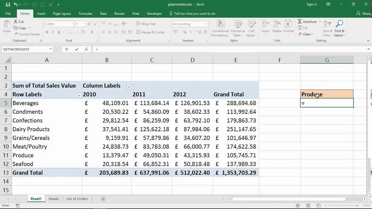
To use Get Pivot Data, you simply need to specify the criteria you want to use for retrieval. This can be done by typing the criteria directly into the formula or by referencing cells that contain the criteria. Once the criteria are defined, the Get Pivot Data function will search the pivot table and extract the corresponding data based on the specified criteria.
One of the key advantages of using Get Pivot Data is that it provides a dynamic way to retrieve data from a pivot table. This means that if any changes are made to the pivot table, such as adding or removing rows or columns, the Get Pivot Data function will automatically update the retrieved data accordingly.
Get Pivot Data also allows for more advanced data retrieval options. You can use operators such as “equal to,” “greater than,” or “less than” to further refine the data extraction. Additionally, you can specify multiple criteria to retrieve data based on multiple conditions. This flexibility gives users a powerful tool for extracting precise and targeted information from their pivot tables.
Overall, Get Pivot Data is a valuable function in Excel that can save you time and effort in retrieving specific data from pivot tables. Understanding how to use it effectively can streamline your data analysis process and help you make more informed business decisions.
Syntax
The syntax for using the “GETPIVOTDATA” function in Excel is as follows:
- Reference: This is the reference to the pivot table from which you want to retrieve data. It can be either a cell reference or a range reference.
- Data Field: Specify the name of the specific data field you want to retrieve. This should be enclosed in double quotation marks.
- Field 1: Choose a field from the pivot table to be used as the filter. This is optional and can be left blank if not needed.
- Item 1: Specify the item from Field 1 that you want to use as a filter. This is optional and can be left blank if not needed.
- Field 2: Select another field to be used as a second filter. This is also optional and can be left blank if not needed.
- Item 2: Specify the item from Field 2 that you want to use as a filter. This is optional and can be left blank if not needed.
- Continue adding Field and Item pairs for additional filters as necessary.
It is important to note that the syntax for the GETPIVOTDATA function is case-sensitive. The reference and data field parameters are mandatory, while the field and item parameters are optional and can be omitted if not required. Also, ensure that the field and item names are entered correctly, as any discrepancy may result in an error or incorrect data retrieval.
Let’s take a look at a few examples to see how the syntax works in practice.
Examples
Here are some examples to help you understand how to use the GETPIVOTDATA function:
Example 1: Suppose you have a pivot table that shows the total sales for each product category and each month. Using the GETPIVOTDATA function, you can easily retrieve specific data points from the pivot table. For example, if you want to get the total sales for the “Electronics” category in the month of January, you can use the following formula: =GETPIVOTDATA(“Sales”,$A$1,”Category”,”Electronics”,”Month”,”January”). This formula will return the total sales amount for the “Electronics” category in January.
Example 2: Let’s say you have a pivot table that shows the number of website visitors based on the country and the referral source. If you want to find out how many visitors came to the website from the United States through the “Google” referral source, you can use the GETPIVOTDATA function. The formula will look like this: =GETPIVOTDATA(“Visitors”,$A$1,”Country”,”United States”,”Referral Source”,”Google”). This formula will give you the number of visitors from the United States who came through the “Google” referral source.
Example 3: In another scenario, let’s say you have a pivot table that displays the average monthly expenses for different departments in a company. If you want to retrieve the average expenses for the Marketing department, you can use the GETPIVOTDATA function. The formula will be: =GETPIVOTDATA(“Expenses”,$A$1,”Department”,”Marketing”). This formula will give you the average monthly expenses for the Marketing department.
Example 4: Suppose you have a pivot table that shows the number of units sold for various products in different regions. If you want to find out the total units sold for a specific product in a particular region, you can use the GETPIVOTDATA function. For example, if you want to get the total units sold for the product “Mobile Phones” in the region “North America,” the formula will be: =GETPIVOTDATA(“Units Sold”,$A$1,”Product”,”Mobile Phones”,”Region”,”North America”). This formula will give you the total units sold for “Mobile Phones” in the “North America” region.
Example 5: Let’s say you have a pivot table that shows the monthly revenue for different product categories and the quarter in which they were sold. If you want to retrieve the revenue for a specific product category and quarter, you can use the GETPIVOTDATA function. For instance, if you want to get the revenue for the “Home Appliances” category in the second quarter, the formula will be: =GETPIVOTDATA(“Revenue”,$A$1,”Category”,”Home Appliances”,”Quarter”,”Q2″). This formula will give you the revenue for the “Home Appliances” category in the second quarter.
These examples should give you a good understanding of how to use the GETPIVOTDATA function to extract data from pivot tables. Remember to adjust the formula based on your specific pivot table structure and data.
Common Errors and Troubleshooting
While using the Get Pivot Data function in Excel, you may encounter a few common errors or issues. Here are some troubleshooting tips to help you resolve them:
Error: #REF!
This error occurs when the reference cell or range that you provided in the formula is not valid. Make sure to double-check the cell references and ensure that they are correct.
Error: #DIV/0!
When you see this error, it means that your formula is trying to divide a number by zero. Check the formula and ensure that you are not dividing by a cell that contains zero.
Error: #N/A!
The #N/A error indicates that the data you are trying to retrieve from the PivotTable does not exist or is not available. Verify that the data exists in the PivotTable and make sure the field names and values are accurate.
Error: #VALUE!
This error occurs when one or more of the arguments in the Get Pivot Data formula are not valid. Check the formula and ensure that all the required arguments are correctly entered.
Error: #NAME?
If you encounter this error, it means that Excel cannot recognize the function name or field name you provided in the formula. Double-check the spelling and ensure that the function name or field name is correct.
Error: #NUM!
This error occurs when the argument provided in the formula is not a valid numeric value. Ensure that all the argument values are numeric and do not contain any non-numeric characters.
Error: #NULL!
The #NULL! error signifies that two ranges in the formula overlap or intersect in an incorrect way. Adjust the ranges and ensure that they do not overlap improperly.
Formula not updating
If you make changes to your PivotTable, such as adding or removing fields, and the Get Pivot Data formula does not update automatically, you may need to refresh the formula. To do so, select the formula cell and press F9 on your keyboard or press the Refresh Data button on the Analyze or Options tab (depending on your Excel version).
By keeping these troubleshooting tips in mind, you can overcome common errors and challenges while using the Get Pivot Data function in Excel. It’s important to double-check your inputs and understand the specific error messages to effectively troubleshoot and resolve any issues that you may encounter.
Conclusion
In conclusion, Get Pivot Data is a powerful tool that can greatly enhance your data analysis and reporting capabilities in Microsoft Excel. By allowing you to extract specific data from pivot tables based on criteria you define, it enables you to generate customized reports and gain valuable insights. Whether you’re a business professional, a data analyst, or a student, mastering Get Pivot Data can save you time and effort in retrieving the information you need.
Remember to keep in mind the tips and techniques mentioned in this article to maximize your efficiency and accuracy when using Get Pivot Data. Practice using different formulas, experiment with various criteria, and gradually increase your understanding of this feature until you become a pivot table expert.
With the knowledge and skills you have acquired, you will be able to navigate large datasets, analyze trends, and make informed decisions with confidence. So, start exploring the endless possibilities of Get Pivot Data today and unleash the full potential of your data analysis tasks!
FAQs
1. What is Get Pivot Data?
Get Pivot Data is a feature in Excel that allows you to retrieve data from a PivotTable by specifying the criteria. It is particularly useful when you want to extract specific information from a PivotTable without manually searching for it.
2. How do I use Get Pivot Data?
To use Get Pivot Data, you need to follow these steps:
– Select a cell in your PivotTable.
– Type the formula “=GETPIVOTDATA(“[field name]“, [PivotTable], [criteria1], [value1], [criteria2], [value2],…)” in a different cell.
– Replace “[field name]” with the name of the field you want to retrieve data from.
– Replace “[PivotTable]” with the reference to your PivotTable.
– Add criteria and their corresponding values to retrieve specific data.
– Press Enter to get the desired result.
3. Can I change the reference to the PivotTable in Get Pivot Data?
Yes, you can change the reference to the PivotTable in Get Pivot Data. Simply click on the cell reference in the formula and select a new range that contains the PivotTable you want to retrieve data from.
4. Can I retrieve data from multiple PivotTables using Get Pivot Data?
No, Get Pivot Data can only retrieve data from one PivotTable at a time. If you want to extract data from multiple PivotTables, you need to use separate formulas for each PivotTable.
5. Can I use wildcards in the criteria of Get Pivot Data?
Yes, you can use wildcards in the criteria of Get Pivot Data. For example, if you want to retrieve data for all entries that start with “A”, you can use the criteria “A*“. The asterisk (*) acts as a wildcard character that represents any number of characters.