
Are you tired of manually rearranging data from rows to columns in Excel? Well, you’re in luck! In this comprehensive guide, we will show you how to easily change data from rows to columns in Excel. Whether you need to pivot your data for analytical purposes, organize survey responses, or simply reformat your data for a specific presentation or report, we’ve got you covered.
Excel provides various techniques and built-in functions that allow you to quickly transform your data layout, saving you time and effort. So, whether you’re a beginner or an intermediate Excel user, this step-by-step tutorial will walk you through the process of converting your data from rows to columns, giving you the freedom to manipulate and analyze your data in a more meaningful way.
So, let’s dive in and discover how you can easily convert your data from rows to columns in Excel!
Inside This Article
- Understanding the Structure of Data in Excel
- Converting Data from Rows to Columns using TRANSPOSE Function
- Using Paste Special to Change Data from Row to Column
- Using Power Query to Transform Data from Row to Column in Excel
- Conclusion
- FAQs
Understanding the Structure of Data in Excel
Excel is a powerful tool that allows you to store and organize data in a structured manner. When working with data in Excel, it is essential to understand the different components of its structure. Excel data is typically organized in a tabular format, with rows and columns. Each row represents a separate record or data entry, while each column represents a specific attribute or data field.
The data in Excel is stored cell by cell, with each cell occupying a unique position in the worksheet. Cells are arranged in a grid-like fashion, with each cell identified by a unique combination of letters and numbers, such as A1, B2, etc. The intersection of a row and a column forms a cell, which can hold different types of data, including numbers, text, dates, and formulas.
Excel utilizes formulas and functions to perform calculations and manipulate data. Formulas are expressions that can be entered into cells to perform mathematical operations or logical evaluations. Functions, on the other hand, are predefined formulas that are designed to perform specific tasks. Excel offers a wide range of functions to handle various data operations, such as summing values, finding averages, and performing text manipulations.”
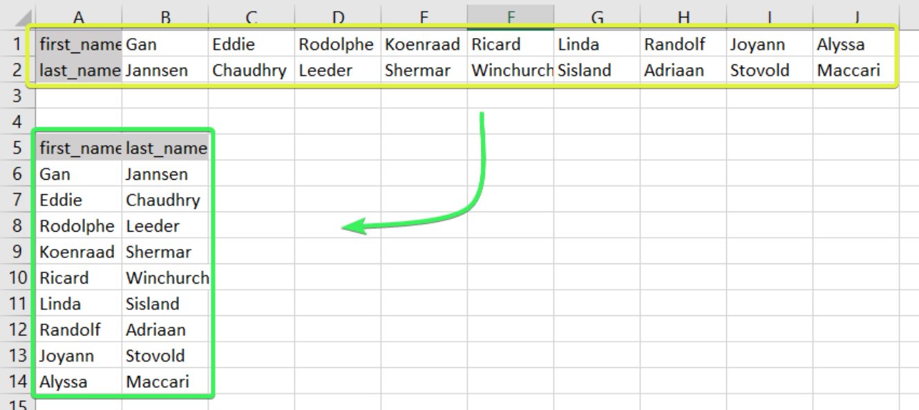
Converting Data from Rows to Columns using TRANSPOSE Function
If you work with Excel frequently, you might have come across situations where you need to convert data from rows to columns. This can be useful when you want to reorganize your data or present it in a different format. Thankfully, Excel provides a built-in function called TRANSPOSE that makes it easy to convert data from rows to columns.
The TRANSPOSE function in Excel allows you to change the orientation of your data by flipping it from rows to columns, or vice versa. It takes an array of cells as input and returns a new array where the rows become columns and the columns become rows.
To use the TRANSPOSE function, follow these steps:
- Select the range of cells that you want to transpose.
- Copy the range by pressing Ctrl+C or right-clicking and selecting “Copy”.
- Select the destination range where you want the transposed data to be placed.
- Right-click on the selected destination range and choose “Paste Special”.
- In the Paste Special dialog box, select the “Transpose” option.
- Click on the “OK” button to complete the transposition.
The TRANSPOSE function can be a handy tool when you have a small dataset that needs to be transposed. However, it’s important to note that it has some limitations. The TRANSPOSE function can only be used on a range of cells that has the same number of rows and columns. If the selected range doesn’t meet this requirement, the TRANSPOSE function will return an error.
Additionally, the TRANSPOSE function is a volatile function, which means that it recalculates every time there is a change in the worksheet. This can potentially slow down the performance of your Excel workbook, especially if you have a large dataset.
Despite its limitations, the TRANSPOSE function can be a powerful tool for quickly converting data from rows to columns in Excel. It can save you time and effort when reorganizing your data or presenting it in a different format.
Using Paste Special to Change Data from Row to Column
If you have a dataset in Excel where the data is arranged in rows and you need to change it to a column format, you can utilize the Paste Special feature. This feature lets you transpose the data, flipping it from rows to columns or vice versa, without the need for complex formulas or functions.
Here’s how you can use Paste Special to change data from row to column:
- Select the range of cells that contain the data you want to transpose.
- Right-click on the selected range and choose the “Copy” option.
- Click on the cell where you want to paste the transposed data.
- Right-click on the cell and choose the “Paste Special” option from the context menu.
- In the Paste Special dialog box, check the “Transpose” checkbox. This will tell Excel to flip the data from rows to columns.
- Click the “OK” button to apply the transpose operation.
By following these steps, you can quickly and easily change the data from row to column format. This method is especially useful when you have a large dataset or when you need to perform calculations or analysis on the transposed data.
It’s important to note that using Paste Special to transpose data only changes its arrangement; it does not affect the values or formulas in the cells. The data will remain the same, just in a different layout.
This technique is handy for reorganizing data for presentation purposes, creating charts, or performing calculations that require data in a column format. By leveraging the Paste Special feature, you can save time and streamline your data manipulation tasks in Excel.
Using Power Query to Transform Data from Row to Column in Excel
Power Query is a powerful tool in Excel that allows you to transform and manipulate data easily. It provides a user-friendly interface to perform various data operations, including changing the data layout from rows to columns. Here’s how you can use Power Query to transform your row-based data into columnar format.
Step 1: Start by selecting your data range. Go to the “Data” tab in Excel and click on “From Table/Range” under the “Get & Transform Data” section. This will open up the Power Query Editor.
Step 2: In the Power Query Editor, you’ll see a preview of your data in a table format. Select the columns that you want to transform from rows to columns. Right-click on the selected columns and choose “Unpivot Columns” from the context menu.
Step 3: The “Unpivot Columns” operation will create two new columns – “Attribute” and “Value.” The “Attribute” column will contain the original column names, and the “Value” column will contain the corresponding values. You can rename these columns if you want by selecting them and using the “Rename” option in the “Transform” tab.
Step 4: Next, you need to pivot the “Attribute” column to convert it into column headers. Select the “Attribute” column and go to the “Transform” tab. Click on the “Pivot Column” option and choose the “Value” column as the values column and the “Attribute” column as the pivot column.
Step 5: After pivoting the column, you’ll see that the data has now been transformed from rows to columns. You can rename the newly created columns by selecting them and using the “Rename” option in the “Transform” tab.
Step 6: Finally, click on the “Close & Load” button to load the transformed data back into Excel. You can choose to load it to a new worksheet or overwrite the existing data if desired.
By following these simple steps, you can use Power Query to easily change the layout of your data from rows to columns in Excel. This feature is particularly helpful when you have datasets that need to be restructured for better analysis or reporting purposes. Power Query enables you to transform your data efficiently and saves you time and effort in manual data manipulation.
In conclusion, learning how to change data from row to column in Excel can significantly enhance your data analysis and reporting capabilities. By using techniques such as the transpose function, copy and paste special, or Power Query, you can quickly transform your data and gain new insights. Whether you need to reorganize survey results, pivot tables, or rearrange data for charts and graphs, Excel provides various methods to accomplish this task.
Mastering this skill allows you to streamline your workflow, save time, and present your data in a more understandable and visually appealing manner. So take the time to explore the different methods mentioned in this article, experiment with your datasets, and become proficient in changing data from row to column. With a solid understanding of these techniques, you can unlock the full potential of Excel for analyzing and reporting data effectively.
FAQs
1. Can you explain how to change data from row to column in Excel?
Certainly! To change data from row to column in Excel, follow these steps:
– Select the row(s) you want to transpose
– Right-click and choose “Copy”
– Select a blank cell where you want the transposed data to start
– Right-click and choose “Paste Special”
– In the Paste Special window, select the “Transpose” option
– Click “OK”
2. Is there a keyboard shortcut for transposing data in Excel?
Yes, there is a keyboard shortcut for transposing data in Excel. After selecting the row(s) you want to transpose, press “Ctrl+C” to copy the data. Then, select a blank cell where you want to paste the transposed data and press “Alt+E+S”, followed by “E”. This will transpose the data.
3. Can I transpose data with formulas in Excel?
Yes, you can transpose data with formulas in Excel. After transposing the data using the steps mentioned above, you can use formulas to perform calculations or manipulate the transposed data.
4. What should I do if my data has headers that I want to transpose as well?
If you want to transpose data with headers, you can follow these steps:
– Copy the headers and the data below them
– Select a blank cell where you want to paste the transposed headers
– Right-click and choose “Paste Special”
– In the Paste Special window, select the “Transpose” option and click “OK”
– Copy the remaining data and paste it starting from the cell below the transposed headers
5. Does changing data from row to column affect the original data?
No, changing data from row to column does not affect the original data. It only rearranges the data in a different orientation without modifying or deleting the original data.