
Are you a frequent user of Microsoft Excel? Do you often find yourself in need of calculating the sum of specific data within a filtered range? If so, you’ve come to the right place! In this article, we will guide you through the process of calculating the sum in Excel with filtered data. Whether you’re a beginner or an experienced user, our step-by-step instructions will help you navigate through this commonly encountered task with ease. From applying filters to selecting the desired data range, we’ll cover all the necessary steps to ensure accurate and efficient calculations. So, let’s dive in and discover how you can leverage Excel’s powerful features to calculate the sum of your filtered data effortlessly!
Inside This Article
- Understanding Filtered Data in Excel
- Methods to Calculate Sum with Filtered Data
- Example: Calculating Sum in Excel with Filtered Data
- Tips and Tricks for Summing Filtered Data in Excel
- Conclusion
- FAQs
Understanding Filtered Data in Excel
Filtered data in Excel refers to the process of selectively displaying a subset of data based on certain criteria. When you apply a filter to a dataset in Excel, you can easily hide or show specific rows that meet the filter conditions. This feature allows you to focus on analyzing or working with a specific subset of data without the distraction of irrelevant information.
Excel provides several filtering options, including simple filtering, advanced filtering, and the use of slicers in pivot tables. Regardless of the filtering method used, the basic concept remains the same: filtering helps you narrow down your data to view only the information that meets your specific requirements.
How Filtering Affects Calculations in Excel
Filtering data in Excel can impact calculations in a few different ways. When you apply a filter, any formulas or functions that reference the filtered data will automatically adjust to consider only the visible cells. This means that calculations such as SUM, AVERAGE, COUNT, and more will reflect the filtered data subset. The filtered data will be temporarily considered as the complete dataset for the purpose of the calculation.
For example, let’s say you have a column of numbers in a filtered dataset and you apply a filter to only show values greater than 10. If you use the SUM function to calculate the sum of this column, the result will only consider the visible cells that meet the filter condition. The SUM function will exclude any hidden or filtered-out cells from the calculation.
It is important to note that Excel provides different functions that can be used to perform calculations specifically on filtered data. These functions consider the hidden or filtered-out cells and provide more accurate results compared to regular functions like SUM or AVERAGE.
Understanding how filtering affects calculations in Excel is crucial to ensure accurate analysis and reporting. It allows you to perform calculations on the subset of data that is relevant to your analysis and avoids including irrelevant or filtered-out data.
To summarize, filtered data in Excel refers to selectively displaying a subset of data based on specific criteria. When you apply a filter, calculations in Excel will adapt to consider only the visible cells that meet the filter conditions. Excel also provides specific functions that can be used to calculate on filtered data accurately.
Methods to Calculate Sum with Filtered Data
When working with Excel, there are several methods you can use to calculate the sum of filtered data. In this article, we will explore two popular methods: using the SUBTOTAL function and applying the SUMIFS function.
Using the SUBTOTAL Function
The SUBTOTAL function is a powerful tool that allows you to perform calculations, such as sums, on data that has been filtered. To use this function, follow these steps:
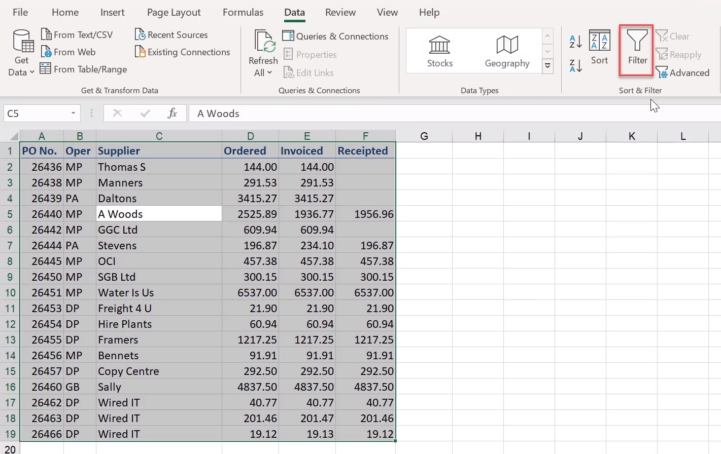
- First, apply the filter to the data range by selecting the data and clicking on the “Filter” button in the “Data” tab.
- Next, select the cell where you want to display the sum.
- Now, enter the following formula in the cell:
=SUBTOTAL(9,filtered_range). The number 9 represents the sum function for SUBTOTAL, and “filtered_range” is the range of cells that have been filtered. - Press Enter, and the cell will show the sum of the filtered data.
This method is useful because it considers only the visible cells after applying the filter. It excludes any hidden cells, making it an accurate calculation for filtered data.
Applying the SUMIFS Function
The SUMIFS function allows you to calculate the sum based on specific criteria in filtered data. This function is particularly handy when you need to sum values that meet multiple conditions. Follow these steps to use the SUMIFS function:
- Begin by applying the filter to the data range, just as you did with the SUBTOTAL method.
- Next, select the cell where you want to display the sum.
- Now, enter the following formula in the cell:
=SUMIFS(sum_range, criteria_range1, criteria1, criteria_range2, criteria2, ...). Replace “sum_range” with the range of cells you want to sum, “criteria_range1” with the first range to apply the criteria, “criteria1” with the first condition, and so on. - Press Enter, and the cell will show the sum based on the specified criteria in the filtered data.
The SUMIFS function is versatile and allows you to sum data based on multiple conditions. It provides a more customized approach to calculating the sum with filtered data.
By using either the SUBTOTAL or SUMIFS function, you can accurately calculate the sum of filtered data in Excel. Remember to apply the filter before using any of these methods to ensure that you are calculating the sum based on the filtered criteria.
Example: Calculating Sum in Excel with Filtered Data
Let’s walk through a step-by-step example on how to calculate the sum in Excel with filtered data. This is a useful technique when you want to perform calculations on a specific subset of your data.
For this example, let’s say you have a sales data table with columns representing the product name, quantity sold, and total sales amount. Your goal is to calculate the total sales amount for a specific product after applying a filter to the data.
1. Start by selecting your data range. In our case, it would be the entire sales data table.
2. Go to the “Data” tab in the Excel ribbon and click on the “Filter” button. This will enable the filter on your selected data range.
3. Now, you will see drop-down arrows appear next to each column header in your table. Click on the arrow for the column that contains the product names.
4. In the drop-down menu, select the specific product you want to calculate the sum for. This will only display the rows in your data that match the selected product.
5. Now, go to an empty cell where you want to display the calculated sum. Let’s say we want to display the sum in cell D2.
6. In cell D2, enter the formula “=SUM(” and then select the range of cells that contains the sales amounts for the filtered data. In our example, it would be the column that contains the total sales amounts.
7. Close the formula with a closing bracket “)” and press Enter. The cell D2 will display the total sum for the filtered data.
That’s it! You have successfully calculated the sum in Excel with filtered data. The result in cell D2 will dynamically update whenever you change the filter or add new data.
Remember, this technique of calculating the sum with filtered data can be applied to other mathematical functions in Excel. Play around with different formula combinations to suit your specific needs.
Tips and Tricks for Summing Filtered Data in Excel
When working with large datasets in Excel, filtering becomes an essential tool to narrow down the data you need for analysis. However, calculating the sum with filtered data can be a bit tricky. In this article, we’ll explore some tips and techniques to accurately calculate the sum with filtered data in Excel, as well as common pitfalls to avoid.
Applying the SUM function with AutoFilter
One of the most straightforward ways to sum filtered data in Excel is by using the SUM function in conjunction with the AutoFilter feature. Here’s how:
- Apply the AutoFilter to your data range by selecting the cells and navigating to the Data tab, then clicking on the Filter button.
- Once you filter your data to display the desired subset, select the cell where you want the sum to appear.
- Enter the SUM function, followed by an opening parenthesis.
- Select the filtered range by clicking and dragging your mouse over the visible cells.
- Close the parenthesis and press Enter to calculate the sum.
This method ensures that only the visible cells in the filtered range are included in the sum calculation.
Using the SUBTOTAL function with filtered data
Another handy function for summing filtered data in Excel is the SUBTOTAL function. This function allows you to perform calculations on visible cells only, even when your data is filtered.
Follow these steps to use the SUBTOTAL function:
- Apply the AutoFilter to your data range as described earlier.
- Select the cell where you want the sum to appear.
- Enter the SUBTOTAL function, followed by an opening parenthesis.
- Specify the function number for sum, which is usually 9. This tells Excel to perform a sum calculation on visible cells.
- Select the filtered range as the argument for the function.
- Close the parenthesis and press Enter to calculate the sum.
By using the SUBTOTAL function with the appropriate function number, you ensure accurate sum calculations even with filtered data.
Utilizing the AGGREGATE function for summing filtered data
The AGGREGATE function is a powerful yet lesser-known function in Excel that allows you to perform various calculations on a range of data, including summing filtered data.
Follow these steps to use the AGGREGATE function:
- Apply the AutoFilter to your data range.
- Select the cell where you want the sum to appear.
- Enter the AGGREGATE function, followed by an opening parenthesis.
- Specify the function number for sum, which is 9.
- Select the filtered range as the argument for the function.
- Close the parenthesis and press Enter to calculate the sum.
The AGGREGATE function offers more flexibility and versatility in performing calculations on filtered data, making it a useful tool for summing in Excel.
Using the DSUM function to calculate sum with specific criteria
If you need to calculate the sum of filtered data based on specific criteria, the DSUM function can come in handy. This function allows you to specify criteria and calculate the sum of a specific column or range that meets the given conditions.
Here’s how to use the DSUM function:
- Ensure your data range has column headers.
- Define the criteria range with column headers and specify the criteria you want to apply.
- Select a cell where you want the sum to appear.
- Enter the DSUM function, followed by an opening parenthesis.
- Select the data range as the database argument.
- Specify the column or range you want to sum in the field argument.
- Specify the criteria range as the criteria argument.
- Close the parenthesis and press Enter to calculate the sum.
The DSUM function allows you to calculate the sum of filtered data based on specific criteria, providing more precise calculations in Excel.
Common pitfalls and mistakes to avoid
When working with filtered data in Excel, there are a few common pitfalls that you should be aware of to ensure accurate sum calculations:
- Forgetting to apply the AutoFilter before attempting to calculate the sum.
- Accidentally including hidden or non-visible cells in the sum calculation.
- Misaligning the ranges or arguments in the formulas, leading to incorrect results.
- Using the wrong function or function number for the calculation type.
- Not updating the sum formula after changing or removing filters.
By being mindful of these common pitfalls, you can avoid mistakes and accurately calculate the sum with filtered data in Excel.
Conclusion
To calculate the sum in Excel with filtered data, you can utilize the SUBTOTAL function along with the filtering feature provided by Excel. This combination allows you to perform calculations on only the visible (filtered) data, making it a powerful tool for data analysis and reporting. By understanding how to use the SUBTOTAL function and how it works with filtered data, you can easily calculate sums, averages, counts, and other important metrics for specific subsets of your data.
Remember to always apply the appropriate filtering before using the SUBTOTAL function to ensure accurate results. By following the steps provided in this guide, you can confidently calculate sums in Excel even with filtered data, unlocking the full potential of this powerful spreadsheet software.
So, whether you’re working with large datasets or simply need to perform calculations on specific subsets of data, Excel’s SUBTOTAL function with filtered data is a valuable tool that can simplify your work and help you gain deeper insights.
FAQs
1. Can I calculate the sum in Excel with filtered data?
Yes, you can calculate the sum in Excel with filtered data. When you apply a filter to your Excel worksheet, only the visible cells are considered for calculations, including the sum.
2. How do I calculate the sum in Excel with filtered data?
To calculate the sum in Excel with filtered data, follow these steps:
- Apply the desired filter to your Excel worksheet.
- Select the cell where you want the sum to appear.
- Use the SUM function to calculate the sum. For example, if you want to sum the values in column A, enter the formula “=SUM(A:A)”.
- Press Enter to get the sum of the filtered data.
3. What happens if I don’t use the SUM function when calculating the sum with filtered data?
If you don’t use the SUM function when calculating the sum with filtered data, Excel will include all the cells in the calculation, even the hidden ones. This will give you an incorrect sum that includes data you may not want to consider.
4. Can I use other functions besides SUM when calculating the sum with filtered data?
Yes, you can use other functions besides SUM when calculating the sum with filtered data. Excel offers a wide range of functions that you can use, such as AVERAGE, MAX, MIN, COUNT, etc. Simply replace the SUM function in the formula with the desired function to calculate the appropriate result.
5. Can I remove the filter after calculating the sum in Excel?
Yes, you can remove the filter after calculating the sum in Excel. To do this, go to the “Data” tab, click on the “Filter” button to toggle off the filter, and the sum will still remain calculated based on the previously filtered data.