How To Change Data In A Pivot Table

If you are working with Microsoft Excel and have ever utilized pivot tables, you may have encountered situations where you need to change the data within the pivot table. Whether it’s updating the source data, modifying calculations, or adjusting the layout, knowing how to efficiently change data in a pivot table is essential for data analysis and reporting. In this article, we will explore various methods to effectively change data in a pivot table, providing you with the tools and knowledge to manipulate your data with ease. Whether you’re a beginner or an experienced Excel user, these tips and techniques will help you streamline your analysis and reporting process, saving you time and effort.

Inside This Article

1. Overview of Pivot Tables
2. Step 1: Opening the Pivot Table
3. Step 2: Modifying the Pivot Table Structure
4. Step 3: Changing the Data Source
5. Step 4: Updating Pivot Table Fields
6. Step 5: Customizing Pivot Table Layout
7. Step 6: Refreshing the Pivot Table Data
8. Step 7: Adding Calculated Fields or Formulas
9. Step 8: Filtering and Sorting Pivot Table Data
10. Step 9: Formatting the Pivot Table
11. Step 10: Saving and Sharing the Modified Pivot Table
12. Conclusion
13. FAQs

Overview of Pivot Tables

A pivot table is a powerful data analysis tool that allows users to summarize and manipulate large sets of data to gain valuable insights. It is particularly useful when dealing with complex or extensive datasets and can be a game-changer for data professionals, analysts, and decision-makers.

Simply put, a pivot table takes raw data and organizes it in a way that is easier to understand and analyze. It enables users to perform calculations, create customized reports, and visualize data in a comprehensive manner.

Pivot tables provide a flexible and dynamic approach to data analysis, allowing users to slice, dice, and summarize information based on different criteria. It offers the ability to quickly and effortlessly rearrange and reorganize data to explore different patterns and trends.

With pivot tables, users can aggregate data, perform calculations, apply filters, sort data, and create personalized reports—all with just a few clicks. This enables them to extract meaningful insights and make data-driven decisions more efficiently and effectively.

Overall, pivot tables are an invaluable tool for data analysis, making complex datasets more manageable and presenting information in a user-friendly, visually appealing manner. They provide a powerful way to explore, understand, and communicate data, empowering users to uncover hidden patterns and trends that can drive business success.

Step 1: Opening the Pivot Table

When working with pivot tables, the first step is to open the pivot table in your preferred software or application. Pivot tables are powerful tools that allow you to analyze and summarize large sets of data with ease.

To open a pivot table, you can follow these simple steps:

1. Open the software or application: Start by launching the software or application where your pivot table is located. This could be Microsoft Excel, Google Sheets, or any other program that supports pivot tables.
2. Open the workbook or file: Once you’ve opened the software, navigate to the specific workbook or file that contains the pivot table you want to work with. You may need to locate the file in your file explorer or use the “Open” option within the software.
3. Select the pivot table: Within the workbook or file, locate the pivot table you want to open. This may involve navigating through different worksheets or tabs if your file contains multiple pivot tables.
4. Click on the pivot table: Once you’ve found the desired pivot table, click on it to select it. This will activate the pivot table and allow you to make changes and modifications to its structure and data.

Opening the pivot table is the first step in the process of modifying and customizing it to suit your analysis needs. By selecting the pivot table within the software or application, you gain access to its various options and functionalities.

Now that you have successfully opened the pivot table, you can move on to the next step in the process: modifying its structure and adjusting the data source. This will allow you to tailor the pivot table to your specific requirements and ensure that it accurately reflects the insights you are seeking.

Step 2: Modifying the Pivot Table Structure

Once you’ve opened your pivot table and reviewed the initial structure, you may find the need to modify it to better suit your data analysis needs. Modifying the pivot table structure allows you to refine and customize how your data is presented and analyzed.

There are several ways to modify the structure of a pivot table. Let’s explore a few key techniques:

1. Adding or removing fields: To modify the structure of your pivot table, you can add or remove fields from the Rows, Columns, or Values areas. Adding fields allows you to further break down and analyze your data, while removing fields can help simplify the pivot table.
2. Moving fields: You can also rearrange the order of fields to change how your data is organized in the pivot table. Simply drag and drop fields within the Rows or Columns areas to reposition them.
3. Modifying field settings: Each field in a pivot table has its own set of settings that can be adjusted. For example, you can change the summary function used for a particular value field or customize the number formatting for a specific field.
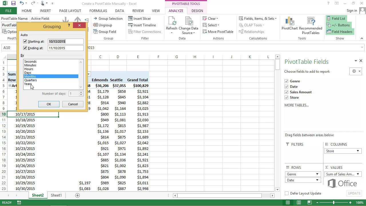
4. Grouping data: If your data contains dates or numerical values that you want to group together, you can use the grouping feature to create custom groups in your pivot table. This can help simplify the analysis and presentation of your data.

Remember, modifying the structure of a pivot table is all about tailoring it to suit your specific data analysis requirements. By adding, removing, moving, and adjusting field settings, you can create a pivot table that provides the insights you need.

Step 3: Changing the Data Source

Changing the data source of a pivot table allows you to update the information it displays without starting from scratch. Whether you have new data to include or need to switch to a different dataset altogether, this step-by-step guide will show you how to seamlessly change the data source in your pivot table.

To begin, open your pivot table by selecting it. You can do this by clicking anywhere inside the pivot table or using the PivotTable Tools on the Excel ribbon.

Next, navigate to the PivotTable Analyze or Options tab, depending on your version of Excel. Look for the “Change Data Source” button or option and click on it.

A dialog box will appear, prompting you to choose the new data source. You have two options: you can either select a range of cells in the same worksheet or specify a different worksheet or workbook entirely.

If you want to select a range of cells in the same worksheet, click on the “Select a Table or Range” option. Use your mouse cursor to highlight the desired cells, and make sure to include all the necessary columns and rows.

If you prefer to use a different worksheet or workbook as your data source, select the “Use an External Data Source” option. You can then browse for the file or specify the connection details, depending on your data source type.

After selecting your new data source, click the “OK” button to confirm and apply the changes. Excel will automatically update the pivot table to reflect the new data.

Keep in mind that changing the data source may alter the structure and behavior of your pivot table. If the new data has different column headers or data types, you may need to adjust the pivot table fields accordingly. Additionally, any calculated fields or formulas you have added may be affected and need to be updated.

It’s worth mentioning that if your pivot table is connected to an external data source, such as a database or an online source, you may need to modify the connection settings instead of changing the data source directly.

By knowing how to change the data source of your pivot table, you can easily update it with new information or switch to a different dataset whenever needed. This flexibility allows you to analyze and present your data in a dynamic and efficient way.

Step 4: Updating Pivot Table Fields

Once you have created a pivot table, you may need to update the fields used in the table to reflect changes in your data. This step-by-step guide will walk you through the process of updating pivot table fields.

The first step is to open the pivot table by selecting the cell within the table. This will activate the PivotTable Tools tab in the Excel ribbon. Click on the “Analyze” tab.

Next, locate the “PivotTable Fields” section. This section displays a list of all the fields used in the pivot table. To update a field, you can simply check or uncheck the corresponding checkbox.

If you want to add a new field to the pivot table, you can do so by dragging the desired field from the “Choose fields to add to report” section into one of the existing areas: “Rows,” “Columns,” or “Values.”

If you want to remove a field from the pivot table, simply uncheck the checkbox next to the field name in the “PivotTable Fields” section. This will remove the field from the pivot table.

Additionally, you have the option to rearrange the order of fields in the pivot table by dragging and dropping them within the “Rows” or “Columns” area. This allows you to customize the layout of your pivot table to suit your needs.

Once you have made the necessary updates to the pivot table fields, you can click on the “Refresh” button in the “Data” group on the “Analyze” tab to update the pivot table data based on the new field selections.

It is important to note that updating the pivot table fields will not modify the original data source. It only affects the display and organization of the data in the pivot table. This allows you to quickly and easily modify the pivot table without making changes to your underlying data.

Updating pivot table fields is a powerful feature that allows you to adapt your pivot table as your data changes. This flexibility makes pivot tables an essential tool for data analysis and reporting in Excel.

Step 5: Customizing Pivot Table Layout

Once you have created a Pivot Table and adjusted its structure and data source, it’s time to move on to the next step: customizing the layout. This step allows you to modify the appearance and arrangement of your Pivot Table to make it more visually appealing and easy to understand.

Here are some key ways to customize the layout of your Pivot Table:

1. Adjusting column width: You can resize the columns in your Pivot Table to ensure that the data is displayed properly. To do this, simply hover over the edge of the column header until the resize cursor appears, then click and drag to adjust the width.
2. Collapsing and expanding fields: If your Pivot Table contains multiple levels of data, you can collapse or expand specific fields to show or hide the details. This can be useful when dealing with large datasets or when you want to focus on specific aspects of the data.
3. Changing row labels: By default, Pivot Tables display row labels using the field names from the data source. However, you can change these labels to make them more user-friendly and meaningful. Simply right-click on a row label, select “Rename Field,” and enter the desired label.
4. Formatting values: You can change the format of the values displayed in your Pivot Table to make them easier to read and understand. This includes options such as setting the number of decimal places, applying currency symbols, and using thousands separators.
5. Selecting different summary functions: Pivot Tables automatically use the sum function to summarize data. However, depending on your analysis needs, you may want to use other summary functions such as average, count, or max. To change the summary function, simply click on the drop-down arrow next to the value field header and select the desired function.
6. Applying conditional formatting: Conditional formatting allows you to highlight specific data points in your Pivot Table based on predefined conditions. For example, you can highlight values that exceed a certain threshold or show trends using color scales. This can help you identify patterns or outliers in your data more easily.
7. Moving and rearranging fields: You can rearrange the fields in your Pivot Table by dragging and dropping them to different sections. This allows you to change the arrangement of rows, columns, and values to present the data in a more meaningful way.

By customizing the layout of your Pivot Table, you can transform it into a powerful data analysis tool that effectively communicates your insights. Experiment with different customization options and find the layout that best suits your needs.

Step 6: Refreshing the Pivot Table Data

After making changes to your pivot table, such as adding or modifying data in the source table, it is important to refresh the pivot table to ensure that the changes are reflected accurately. Refreshing the pivot table updates the data and calculations within the table, allowing you to view the most recent information.

To refresh the pivot table data, follow these steps:

1. Click anywhere within the pivot table to activate it.
2. Go to the “PivotTable Analyze” or “Options” tab in the Excel ribbon.
3. In the “Data” group, locate the “Refresh” button.
4. Click on the “Refresh” button.

Alternatively, you can right-click anywhere within the pivot table, and select “Refresh” from the context menu. This will also update the data in the pivot table.

When you refresh the pivot table data, Excel will retrieve the updated information from the source table and recalculate any formulas or calculations within the pivot table. This ensures that you have the most accurate and up-to-date analysis.

It is important to note that if the source data has been modified significantly, such as adding or removing columns, it may be necessary to adjust the pivot table structure or reselect the data source to ensure accurate refreshing of the data.

Keep in mind that refreshing the pivot table data is particularly useful if you are working with dynamic data that changes frequently. By refreshing the pivot table, you can quickly and easily update your analysis without having to manually make changes.

Additionally, if you have multiple pivot tables in your workbook that are based on the same data source, refreshing one pivot table will automatically update all the other pivot tables, ensuring consistency across your analysis.

Overall, refreshing the pivot table data is an essential step in maintaining the accuracy and relevance of your analysis. By following these simple steps, you can easily update your pivot table and stay up to date with the latest information.

Step 7: Adding Calculated Fields or Formulas

One of the powerful features of Pivot Tables is the ability to create calculated fields or formulas. Calculated fields allow you to perform calculations using the existing data in the Pivot Table. This can be extremely useful when you need to analyze and derive insights from your data in a more customized way.

To add a calculated field, follow these steps:

1. Ensure that your Pivot Table is selected or activated.
2. Go to the “PivotTable Tools” tab in the ribbon and click on the “Options” or “Analyze” tab.
3. In the “Calculations” group, click on the “Fields, Items, & Sets” button and select “Calculated Field”.
4. In the “Name” field, enter a name for your calculated field.
5. In the “Formula” field, enter the formula you want to use. You can use operators like +, -, *, /, as well as functions like SUM, AVERAGE, COUNT, etc.
6. Click “Add” to add the calculated field to your Pivot Table.

Once you have added the calculated field, it will appear as a new field in your Pivot Table field list. You can now use it as you would any other field in the Pivot Table. Remember that the calculated field will update automatically whenever you refresh the Pivot Table or update the underlying data.

Calculated fields can be particularly useful when you want to perform complex calculations or create customized metrics based on existing data. For example, you can create a calculated field to calculate the profit margin by dividing the profit by the sales, or you can create a calculated field to calculate the year-over-year growth rate.

It’s important to note that adding calculated fields may increase the complexity of your Pivot Table, so make sure to test and validate your formulas to ensure the accuracy of your analysis.

Adding calculated fields or formulas gives you the flexibility to analyze and manipulate your data in a way that suits your specific needs. Experiment with different formulas and calculations to uncover valuable insights from your Pivot Table.

Step 8: Filtering and Sorting Pivot Table Data

Filtering and sorting data in a pivot table allows you to analyze and visualize the information in a more focused and organized manner. By applying filters and sorting options, you can quickly identify trends, outliers, and patterns within your data.

To filter the data in a pivot table, you can use the filter buttons located next to each field in the pivot table’s field list. These buttons provide a convenient way to select specific data points or apply custom criteria to focus on the relevant information.

For example, if you have a pivot table that shows sales data by region, you can use the filter buttons to easily select a specific region or multiple regions to analyze. This allows you to drill down into the details of the selected region(s) without cluttering the pivot table with unnecessary data.

In addition to filtering, you can also sort the data in a pivot table to arrange it in a specific order. Sorting can be done in ascending or descending order based on the values in a particular field. This can be helpful when you want to identify the top or bottom performers, analyze trends, or compare data between different categories.

To sort the data in a pivot table, you can click on the column header of the field you want to sort by. This will arrange the data in either ascending or descending order, depending on the initial click. Subsequent clicks on the same column header will toggle between the two sorting options.

Furthermore, you have the option to add multiple levels of sorting to further refine the data arrangement. This can be accomplished by holding the Shift key while clicking on the additional column headers in the desired order.

By combining filtering and sorting techniques, you can gain valuable insights and make data-driven decisions based on the specific criteria and patterns you are interested in analyzing.

Remember, filtering and sorting in a pivot table are dynamic features, which means you can easily modify them as needed. You can remove filters, change filter criteria, switch sorting orders, or add/remove sorting levels to adapt to your evolving analytical needs.

Utilize the power of filtering and sorting in pivot tables to streamline your data analysis process, uncover meaningful insights, and make informed decisions.

Step 9: Formatting the Pivot Table

Formatting is an essential step when working with pivot tables as it allows you to customize the appearance of your data and make it more visually appealing. In this step, we will explore various formatting options that can enhance the readability and presentation of your pivot table.

1. Apply Cell Formatting: You can format individual cells or ranges of cells in your pivot table to emphasize important data or highlight specific values. Right-click on a cell, select “Format Cells,” and choose the desired formatting options such as font style, color, size, borders, or fill color.

2. Format Column Width: Adjusting the column width ensures that your data is displayed properly without any truncation. To do this, hover your cursor over the column header boundary until it changes to a double-sided arrow. Click and drag to the desired width for each column.

3. Modify Row Height: Similar to adjusting column width, you can modify the row height to accommodate larger text or prevent overlapping of data. Hover your cursor over the row header boundary until it changes to a double-sided arrow. Click and drag to adjust the height of each row.

4. Change Number Formatting: Pivot tables often display numerical data, and you may want to format them based on your preference. Right-click on a cell containing numerical data, select “Number Format,” and choose from various options such as currency, percentage, date, or custom formats.

5. Apply Conditional Formatting: Conditional formatting allows you to apply different formatting styles to cells based on certain conditions. It helps highlight patterns, trends, or specific values in your data. To apply conditional formatting, select the desired cell range, go to the “Home” tab, and choose from available formatting rules.

6. Add Borders and Gridlines: Adding borders and gridlines can improve the visual clarity of your pivot table. To add borders, select the cell range, right-click, choose “Format Cells,” go to the “Border” tab, and select the desired border styles. To display gridlines, go to the “View” tab and check the “Gridlines” option.

7. Use Cell Styles: Excel offers a variety of predefined cell styles that allow you to quickly apply a consistent formatting theme across your pivot table. To access cell styles, go to the “Home” tab, and select from the available styles in the “Styles” group.

8. Apply Conditional Formatting Icon Sets: Icon sets are a powerful way to visualize data using icons based on the cell values. You can highlight trends, variances, or performance indicators using different icons. Select the range of cells, go to the “Home” tab, and choose the desired icon set from the conditional formatting options.

9. Adjust Font Styles and Colors: Customizing the font styles and colors can help improve the readability and overall aesthetics of your pivot table. Select the cells or range you want to modify, go to the “Home” tab, and choose the desired font, font size, or font color options.

10. Hide or Show Grand Total and Subtotals: Sometimes, you may want to hide the grand total or subtotals in your pivot table to focus on specific data. Right-click on the pivot table, select “PivotTable Options,” go to the “Totals & Filters” tab, and choose the appropriate options to show or hide the desired totals.

By applying these formatting techniques, you can transform your pivot table into a visually appealing and easy-to-read data analysis tool.

Step 10: Saving and Sharing the Modified Pivot Table

Once you have made all the desired changes to your pivot table, it’s important to save and share it so that others can benefit from your insights. Here are a few steps to guide you in saving and sharing your modified pivot table:

1. Save the Workbook: Before saving the pivot table, make sure to save the entire workbook. This ensures that all changes, including the modified pivot table, are preserved. To save the workbook, click on the File menu, select Save or Save As, and choose a location to save the file.

2. Update Data Source: If your pivot table is connected to an external data source, such as a database or an Excel spreadsheet, ensure that the data source is up to date. Refresh the data source to reflect any recent changes, ensuring that your pivot table is based on the most current information.

3. Save the Pivot Table: To specifically save the modified pivot table, right-click anywhere within the pivot table, select PivotTable Options, and choose the Save PivotTable option. Give it a meaningful name and choose the location to save the file.

4. Share the Pivot Table: There are various ways to share the modified pivot table with others. You can send the file via email or a file-sharing platform, such as Google Drive or Dropbox. Another option is to publish the pivot table to a web page or a shared network location and grant access to the intended recipients.

5. Consider Sharing as PDF: If you want to ensure that the formatting and layout of the pivot table remain intact, consider saving and sharing it as a PDF file. This way, anyone opening the file will see the pivot table exactly as you intended, without the risk of data or formatting being inadvertently changed.

6. Communicate Key Findings: When sharing the modified pivot table, it’s helpful to provide a brief summary or key findings that highlight the main insights gained from the data analysis. This will provide context and make it easier for recipients to understand and interpret the information presented in the pivot table.

By following these steps, you can effectively save and share the modified pivot table, allowing others to benefit from your data analysis and insights. Remember to regularly update and refresh the pivot table as new data becomes available to ensure its accuracy and relevance.

In conclusion, understanding how to change data in a pivot table is a valuable skill that can greatly enhance your data analysis capabilities. By being able to manipulate and update the data within a pivot table, you can extract meaningful insights and make informed decisions. Whether you need to add or remove data, make adjustments to calculations, or refresh your pivot table with updated information, the ability to make these changes will empower you to explore your data more effectively. Remember to evaluate the impact of any changes you make to ensure the integrity and accuracy of your analysis. With a solid understanding of how to change data in a pivot table, you’ll be well-equipped to navigate the ever-changing landscape of data and unlock its full potential.

FAQs

1. Can I change the source data of a pivot table?
Yes, you can change the source data of a pivot table. You can modify the data range or update the data in the source range, and the pivot table will reflect the changes accordingly.

2. How do I update the data range of a pivot table?
To update the data range of a pivot table, follow these steps:

1. Select any cell within the pivot table.
2. On the Ribbon, go to the “PivotTable Analyze” or “Options” tab, depending on your Excel version.
3. Click on the “Change Data Source” button.
4. Select the new data range for your pivot table.
5. Click “OK” to update the data range.

3. Can I add or remove fields in a pivot table?
Absolutely! You can add or remove fields in a pivot table to customize the presentation of your data. To add a field, simply drag and drop it into one of the pivot table areas (rows, columns, values, or filters). To remove a field, drag it out of the pivot table or uncheck it from the field list.

4. How do I change the summary function for a specific field?
To change the summary function for a specific field in a pivot table, follow these steps:

1. Select any cell within the pivot table.
2. On the Ribbon, go to the “PivotTable Analyze” or “Options” tab, depending on your Excel version.
3. Click on the “Value Field Setting” or “Field Settings” button.
4. In the dialog box, select the field you want to change and click on the “Summarize Value By” dropdown.
5. Select the desired summary function, such as sum, average, count, etc.
6. Click “OK” to apply the change.

5. Can I rearrange the layout of a pivot table?
Yes, you can rearrange the layout of a pivot table by dragging and dropping fields in the PivotTable Field List or by right-clicking on a field and selecting options like “Move Up” or “Move Down.” This way, you can reorganize the rows, columns, and values to present your data in different ways.