
If you’re looking to add a bit of flair to your data visualization in Excel, you may have wondered how to change the shape of data points. While Excel provides a default shape for data points in charts, it’s possible to customize them to suit your needs and make your charts stand out.
By changing the shape of data points, you can enhance the visual impact of your charts, highlight specific data points, or differentiate between different categories within your data. Whether you’re creating a line graph, scatter plot, or bar chart, Excel offers a range of options to choose from.
In this article, we’ll guide you through the process of changing the shape of data points in Excel, explaining the steps involved and offering some tips and tricks along the way. So, let’s dive in and transform how your data points appear in your Excel charts!
Inside This Article
- Methods for Changing Data Point Shapes in Excel
- Ways to Modify Data Point Shapes Using Formatting Options
- How to Customize Data Point Shapes in Excel
- Conclusion
- FAQs
Methods for Changing Data Point Shapes in Excel
When it comes to visualizing data in Excel, you have several options for customizing your charts and graphs. One aspect you might want to modify is the shape of the data points. In Excel, data points are the individual markers or symbols that represent the data on your chart. By changing their shapes, you can add style and visual interest to your data visualizations.
There are a few methods you can use to change the shape of data points in Excel, depending on the type of chart or graph you are working with. Let’s explore some of these methods below:
Scatter Plot
If you’re working with a scatter plot, which is a chart that displays the relationship between two sets of numerical data, you have the option to change the shape of the data points. Excel provides a variety of built-in shapes to choose from, including circles, squares, triangles, diamonds, and more. To change the shape of the data points in a scatter plot, simply select the data series, right-click, and choose “Format Data Series.” From there, you can navigate to the “Marker Options” tab and select the desired shape.
Bubble Chart
For bubble charts, which display three-dimensional data using varying sizes and colors, you can also change the shape of the data points. In addition to the built-in shapes mentioned earlier, Excel offers additional options specifically designed for bubble charts, such as cylinders, cones, and wedges. To modify the shape of the data points in a bubble chart, follow the same steps as described for scatter plots.
Changing Marker Style
In some cases, you may want to change the style of the marker itself, rather than just the shape. Excel provides various options to customize the appearance of the marker, including changing the fill color, outline color, and border thickness. This can be done by selecting the data series, right-clicking, and choosing “Format Data Series.” Navigate to the “Marker Options” or “Marker Fill” tab, depending on your version of Excel, to access these customization options.
Adjusting Marker Size
In addition to changing the shape and style of the markers, you can also adjust their size to make them more visually prominent or subtle. By resizing the data points, you can emphasize certain areas of your chart or create a more balanced and cohesive look. To change the size of the markers, select the data series, right-click, and choose “Format Data Series.” From there, navigate to the “Marker Options” tab and adjust the marker size using the provided options.
By utilizing these methods, you can take your Excel charts and graphs to the next level by customizing the shape of the data points. Experiment with different shapes, styles, and sizes to find the visual representation that best fits your data and enhances its impact. With a bit of creativity and customization, you can create visually appealing and engaging data visualizations in Excel.
Ways to Modify Data Point Shapes Using Formatting Options
When working with data in Excel, it is essential to present it in a visually appealing way that effectively communicates the information. One way to enhance the visual impact of your data is by modifying the shapes of data points within your charts. Excel provides several formatting options that allow you to customize the appearance of data markers, such as scatter plots and bubble charts.
Here are some ways you can modify the shape of data points in Excel:
1. Using Scatter Plots: Scatter plots are an excellent choice for displaying data points in two dimensions. To modify the shape of data points in a scatter plot, follow these steps:
– Select the scatter plot chart.
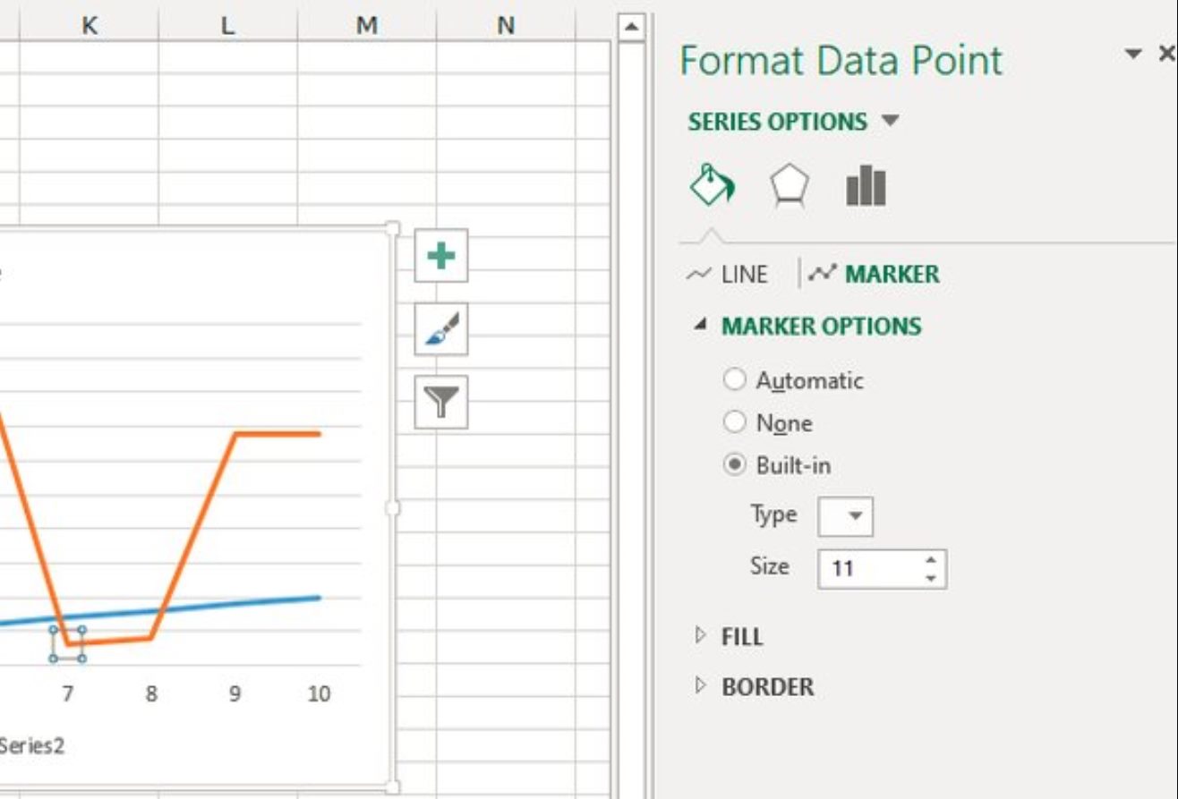
– Right-click on a data point and choose “Format Data Point” from the context menu.
– In the Format Data Point pane, go to the “Marker Options” tab.
– Under “Marker Type,” select the desired shape for the data points, such as a circle, square, or diamond.
– Customize other formatting options like size, fill color, and border color to further enhance the appearance.
2. Using Bubble Charts: Bubble charts are ideal for visualizing data points with three dimensions, where the size of the marker represents a third variable. To modify the shape of data points in a bubble chart, follow these steps:
– Select the bubble chart.
– Right-click on a data point and choose “Format Data Point” from the context menu.
– In the Format Data Point pane, go to the “Marker Options” tab.
– Under “Marker Type,” choose the desired shape for the data points.
– Customize other formatting options like size, fill color, and border color to enhance the visual impact.
3. Changing Marker Style: Excel provides various marker styles that can be applied to data points in charts. To change the marker style, follow these steps:
– Select the chart and go to the “Design” tab in the Excel ribbon.
– Click on the “Change Chart Type” button.
– In the “Change Chart Type” dialog box, select the desired chart type, such as a scatter plot or a bubble chart.
– Click on the “Marker” tab and choose the marker style that best suits your needs.
4. Adjusting Marker Size: The size of data points can be modified to highlight specific values or emphasize certain data points. To adjust the marker size, follow these steps:
– Select the chart and go to the “Format” tab in the Excel ribbon.
– Use the “Marker Size” option to increase or decrease the size of the data points.
– Experiment with different sizes until you achieve the desired visual effect.
By utilizing these formatting options in Excel, you can transform your data points into visually appealing shapes that help convey your message effectively. So, don’t be afraid to experiment with different markers, sizes, and styles to create charts that stand out and capture your audience’s attention.
How to Customize Data Point Shapes in Excel
Excel is a powerful tool for data analysis and visualization, and one of its notable features is the ability to customize the shape of data points in charts. By changing the shape of data points, you can add a visual element to your charts that enhances their overall appearance and helps convey the information more effectively. In this article, we will explore how to customize data point shapes in Excel and make your charts stand out.
There are various ways to customize the shape of data points in Excel, depending on the type of chart you are working with. Let’s take a look at some of the most commonly used chart types and how to customize their data point shapes.
Scatter Plot
A scatter plot is a great chart type for visualizing the relationship between two sets of data. To customize the data point shapes in a scatter plot, follow these steps:
- Select the data points in the scatter plot by clicking on any individual data point.
- Right-click on one of the selected data points and choose “Format Data Series” from the context menu.
- In the Format Data Series pane, go to the “Marker Options” tab.
- Under “Marker Type,” choose the desired shape from the drop-down menu.
- Adjust the size and color of the data points as needed.
Bubble Chart
A bubble chart is similar to a scatter plot but includes a third dimension, represented by the size of the data points. To customize the shape of data points in a bubble chart, follow these steps:
- Select the data points in the bubble chart by clicking on any individual data point.
- Right-click on one of the selected data points and choose “Format Data Series” from the context menu.
- In the Format Data Series pane, go to the “Marker Options” tab.
- Under “Marker Type,” choose the desired shape from the drop-down menu.
- Adjust the size and color of the data points as needed.
Changing Marker Style
In addition to changing the basic shape of data points, Excel also allows you to customize the marker style for different data series. This can be useful when you have multiple data series in a chart and want to distinguish them visually. To change the marker style, follow these steps:
- Select the data series in the chart by clicking on one of the data points in the series.
- Right-click on the selected data series and choose “Format Data Series” from the context menu.
- In the Format Data Series pane, go to the “Marker Options” tab.
- Under “Marker Style,” choose the desired style from the drop-down menu.
Adjusting Marker Size
Excel also gives you control over the size of data points in your charts. By adjusting the marker size, you can emphasize certain data points or make them more visually appealing. Here’s how to adjust the marker size:
- Select the data points in the chart by clicking on any individual data point.
- Right-click on one of the selected data points and choose “Format Data Series” from the context menu.
- In the Format Data Series pane, go to the “Marker Options” tab.
- Under “Marker Size,” adjust the size using the slider or enter a specific value.
With these steps, you can easily customize the shape, style, and size of data points in Excel charts to create visually compelling and informative visualizations. Experiment with different options to find the best representation for your data and make your charts truly stand out.
Conclusion
Changing the shape of data points in Excel can greatly enhance the visual impact of your charts and graphs. By utilizing the various customization options available, you can effectively convey your data in a more engaging and visually appealing manner.
Whether you want to emphasize certain data points or create a unique visual representation, Excel provides a range of tools to modify the shape of your data points. From simple circles and squares to complex shapes and symbols, you have the flexibility to make your charts truly stand out.
Remember, selecting the right shape and size for your data points is crucial to effectively communicate your message. Experiment with different options and pay attention to the overall aesthetics of your charts.
So, the next time you want to make your data visualization more impactful, don’t hesitate to explore the shape customization features in Excel. Let your creativity shine and transform your charts into dynamic and captivating representations of your data!
FAQs
1. Can I change the shape of individual data points in Excel?
Yes, you can change the shape of individual data points in Excel. It allows you to visually represent data in different shapes such as circles, squares, diamonds, triangles, and more.
2. How can I change the shape of data points in Excel?
To change the shape of data points in Excel, follow these steps:
- Select the chart that contains the data points you want to change.
- Right-click on an individual data point and select “Format Data Point” or “Format Data Series” from the context menu.
- In the Format Data Point or Format Data Series pane, navigate to the “Marker Options” or “Marker Style” section.
- Choose the desired shape for the data points from the available options.
3. Are there any limitations to changing the shape of data points in Excel?
While Excel offers various shapes for data points, it is important to note that not all chart types support changing the shape of data points. Additionally, certain versions of Excel may have limitations on the available shapes.
4. Can I customize the appearance of the data points with different colors or sizes?
Yes, you can customize the appearance of the data points in Excel. In addition to changing the shape, you can also modify the color, size, and other visual aspects of the data points to create visually appealing charts.
5. Will changing the shape of data points affect the accuracy of my charts?
Changing the shape of data points does not impact the accuracy of your charts. It is purely a visual customization option that allows you to better represent data in a way that suits your needs.