
Excel is a powerful tool that many of us rely on for managing and analyzing data. Whether you’re working with spreadsheets, charts, or graphs, Excel provides a wealth of features to help you make sense of your data. One common task that you may come across is the need to switch the data axis in Excel.
Switching the data axis involves changing the orientation of your data from rows to columns, or vice versa. This can be particularly useful when you want to rearrange your data to better visualize trends or compare different sets of data. In this article, we will explore the steps to switch data axis in Excel, providing you with a comprehensive guide to help you manipulate your data and create more effective visualizations.
Inside This Article
- Method 1: Using the “Switch Row/Column” Feature
- Method 2: Transposing the Data
- Method 3: Using the “Paste Special” Feature
- Method 4: Manually Reorganizing the Data
- Conclusion
- FAQs
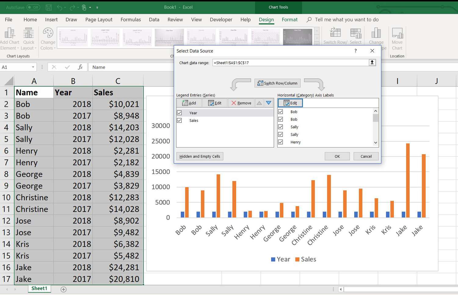
Method 1: Using the “Switch Row/Column” Feature
One of the easiest ways to switch the data axis in Excel is by utilizing the “Switch Row/Column” feature. This feature allows you to interchange the position of rows and columns in your data table, ultimately changing the data axis. Follow these simple steps to use this feature:
- Open your Excel worksheet and select the data range that you want to switch.
- Right-click on the selected range and choose the “Copy” option, or use the shortcut key Ctrl + C.
- Next, right-click on the cell where you want to paste the transposed data and select the “Paste Special” option from the context menu, or use the shortcut key Ctrl + Alt + V.
- In the “Paste Special” dialog box, check the “Transpose” option.
- Click on the “OK” button to complete the process.
By following these steps, your data axis will be switched, and the data that was previously arranged in rows will now be in columns, and vice versa. This method is quick and effective when you need to rearrange the data axis in your Excel worksheet.
Method 2: Transposing the Data
If you want to switch the data axis in Excel, one effective method is to use the “Transpose” feature. Transposing the data allows you to interchange the rows and columns, effectively flipping the data axis. This can be particularly useful when you want to present your data in a different format or analyze it from a different perspective.
To transpose the data in Excel, follow these simple steps:
- Select the range of data that you want to transpose. This can be a single row or column, or a range of cells.
- Copy the selected data by pressing Ctrl+C or right-clicking and choosing “Copy” from the context menu.
- Navigate to the cell where you want to paste the transposed data. Make sure the cell is outside the range of the original data.
- Right-click on the destination cell and choose “Paste Special” from the context menu.
- In the “Paste Special” dialog box, check the “Transpose” option. This tells Excel to transpose the copied data when pasting it.
- Click “OK” to apply the transposition and paste the data.
By following these steps, you can easily switch the data axis in Excel using the transposition method. This feature is especially useful when you want to convert rows into columns or vice versa, making it easier to analyze and present your data in different formats.
Method 3: Using the “Paste Special” Feature
Another way to switch the data axis in Excel is by using the “Paste Special” feature. This method allows you to transpose the data quickly and easily. Here’s how to do it:
1. Copy the data range that you want to switch. You can do this by selecting the cells and pressing Ctrl+C or right-clicking and selecting “Copy”.
2. Select the cell where you want to transpose the data. This should be the top-left cell of the new range.
3. Right-click on the selected cell and choose “Paste Special” from the context menu.
4. In the “Paste Special” dialog box, check the “Transpose” option under the “Paste” section.
5. Click on the “OK” button to complete the transpose operation. The data will now be switched to the desired axis in the selected range.
This method works well when you have a large data range and want to switch the rows and columns quickly. It saves you time and effort compared to manually reorganizing the data.
Note that using the “Paste Special” feature transposes the data, so it replaces the original data with the transposed data. If you want to keep the original data, make sure to copy and paste it into a different location before using the “Paste Special” feature.
By using this method, you can easily switch the data axis in Excel and manipulate your data in the desired format. It is a handy feature that can make your data analysis and presentation more efficient.
Method 4: Manually Reorganizing the Data
If the previous methods mentioned above don’t work for you or if you prefer a more hands-on approach, you can manually reorganize the data in Excel. This method allows you to have full control over how the data is arranged.
To manually reorganize the data, follow these steps:
- Select the data you want to rearrange. You can do this by clicking and dragging over the cells that contain the data.
- Cut or copy the selected data. You can do this by right-clicking on the selected cells, choosing the “Cut” or “Copy” option from the context menu, or using the keyboard shortcuts (Ctrl+X for Cut, Ctrl+C for Copy).
- Select the destination where you want to paste the data. Make sure that the destination cells have enough space to accommodate the pasted data.
- Paste the data into the new location. You can do this by right-clicking on the destination cells and choosing the “Paste” option from the context menu, or using the keyboard shortcuts (Ctrl+V for Paste).
- Adjust the formatting and layout as necessary. This step is important to ensure that the pasted data fits well and looks organized in the new location.
By manually reorganizing the data, you have the flexibility to arrange it in any way you want. You can change the order of rows and columns, group related data together, and create a customized layout that suits your needs.
However, it’s worth mentioning that manually reorganizing the data can be time-consuming, especially if you’re working with a large dataset. Therefore, it’s recommended to use this method for smaller datasets or when you require precise control over the arrangement of the data.
Conclusion
In conclusion, being able to switch data axis in Excel is a valuable skill that can greatly enhance your data analysis and visualization capabilities. By rearranging the data on the axis, you can gain new insights and present your information in a more meaningful way. Whether you want to compare different categories, analyze trends over time, or highlight specific data points, Excel provides a variety of options to customize your charts and graphs.
Remember to carefully consider the type of data you have and the message you want to convey when deciding on the most appropriate axis arrangement. Experiment with different configurations and leverage the functionality of Excel to create compelling visual representations of your data.
With the knowledge and techniques outlined in this guide, you can confidently switch data axis in Excel and unlock the full potential of your data. So go ahead, explore the possibilities, and take your data analysis and visualization skills to the next level.
FAQs
1. How do I switch the data axis in Excel?
To switch the data axis in Excel, you can follow these steps:
- Select the chart you want to modify.
- Click on the “Chart Elements” button (represented by a plus icon) on the upper-right corner of the chart.
- From the dropdown menu, check the box for “Axis Titles” and select the desired axis you want to switch.
- Right-click on the axis title and choose “Format Axis Title” from the context menu.
- In the Format Axis Title pane, choose the option “Rotate 270 degrees” or “Rotate 90 degrees” to switch the axis orientation.
- Click “Close” to apply the changes.
2. Can I switch the data axis in Excel with a keyboard shortcut?
Unfortunately, there is no specific keyboard shortcut to switch the data axis in Excel. You will need to follow the steps mentioned above using the mouse and the appropriate menus.
3. What is the purpose of switching the data axis in Excel?
Switching the data axis in Excel allows you to change the orientation of the axis labels, making your chart more readable or aligning it with your data presentation requirements. It can help to highlight different aspects of your data, compare different data sets, or emphasize specific categories or values.
4. Can I switch the data axis in Excel for different chart types?
Yes, you can switch the data axis for various chart types in Excel, including bar charts, column charts, line charts, scatter plots, and more. The process to switch the data axis remains the same regardless of the chart type.
5. Are there any limitations or considerations when switching the data axis in Excel?
When switching the data axis in Excel, you should consider the readability and interpretation of your chart. Ensure that the data is still easily understood and that the labels or values are not overlapping or obscured. It’s also essential to evaluate the impact of the axis switch on the overall chart presentation and the message you want to convey to your audience.