How To Use Slicers To Filter Data In Excel

Excel is a powerful tool, and knowing how to efficiently manage and manipulate data within it can greatly enhance productivity. One useful feature in Excel is the ability to use slicers to filter data. Slicers provide an intuitive and user-friendly way to visually filter data, making it easier to analyze and understand the information present in your Excel spreadsheets.

Whether you’re a beginner or an experienced Excel user, learning how to effectively use slicers can help you save time and simplify data analysis. In this article, we will explore the ins and outs of using slicers in Excel. We’ll cover everything from how to insert slicers, connect them to data tables, and customize their appearance. By the end, you’ll have the knowledge and tools to confidently filter your data using slicers, empowering you to gain valuable insights from your Excel spreadsheets.

Inside This Article

1. Overview
2. Setting up Slicers in Excel
3. Using Slicers to filter data
4. Customizing and managing Slicers
5. Conclusion
6. FAQs

Overview

Slicers are a powerful feature in Excel that allow you to easily filter data in your spreadsheets. They provide a user-friendly way to visually select and view specific data subsets, making it much simpler to analyze and present information. With slicers, you can filter tables, PivotTables, and PivotCharts with just a few clicks, without the need for complex formulas or manual filtering.

Slicers were introduced in Excel 2010 and have quickly become a favorite tool among data analysts and Excel users. They provide an intuitive and interactive way to explore data and identify trends or patterns. Whether you are working with a small dataset or a large database, slicers can help you streamline your data analysis process and make it more efficient and effective.

In this article, we will delve into the world of slicers and learn how to set them up, use them to filter data, and customize them to fit your specific needs. So let’s get started and discover the power of slicers in Excel!

Setting up Slicers in Excel

If you’re looking to efficiently filter and navigate through large sets of data in Excel, Slicers can be a valuable tool. Slicers provide a user-friendly interface that allows you to easily control and manipulate data without the need for complex formulas or filters. With just a few simple steps, you can set up Slicers in Excel and enhance your data analysis experience.

To begin, make sure you have a data table or pivot table in Excel that you want to filter using Slicers. Once you have your dataset ready, follow these steps:

1. Select the cell or range of cells that you want to associate with the Slicer. This can be a single column or multiple columns.
2. Head over to the “Insert” tab in the Excel ribbon, and click on the “Slicer” button in the “Filters” group. A dialog box will appear.
3. In the dialog box, choose the column(s) that you want to use as Slicers. You can select multiple columns by holding down “Ctrl” or “Shift” while clicking on the column names. Click “OK” to proceed.
4. Excel will automatically insert the Slicer(s) as a new separate object. You can move and resize the Slicer(s) as needed to fit your worksheet layout.
5. Finally, simply click on the Slicer buttons to filter the associated data. You can select multiple options within a Slicer by holding down “Ctrl” while clicking. To clear a filter, click on the “Clear Filter” button in the top-right corner of the Slicer.

That’s it! You have successfully set up Slicers in Excel. Now you can easily filter and navigate through your data without the hassle of complex formulas or filters.

Remember, Slicers provide an intuitive way to interact with your data, making it easier to analyze and visualize trends. By incorporating Slicers into your Excel workflow, you can streamline your data analysis process and make more informed decisions.

Using Slicers to filter data

One of the most powerful features in Excel for data analysis is the Slicer tool. Slicers allow you to easily filter data in a visually appealing way, making it quick and efficient to analyze and manipulate large datasets. With just a few clicks, you can instantly narrow down your data to focus on specific criteria or categories.

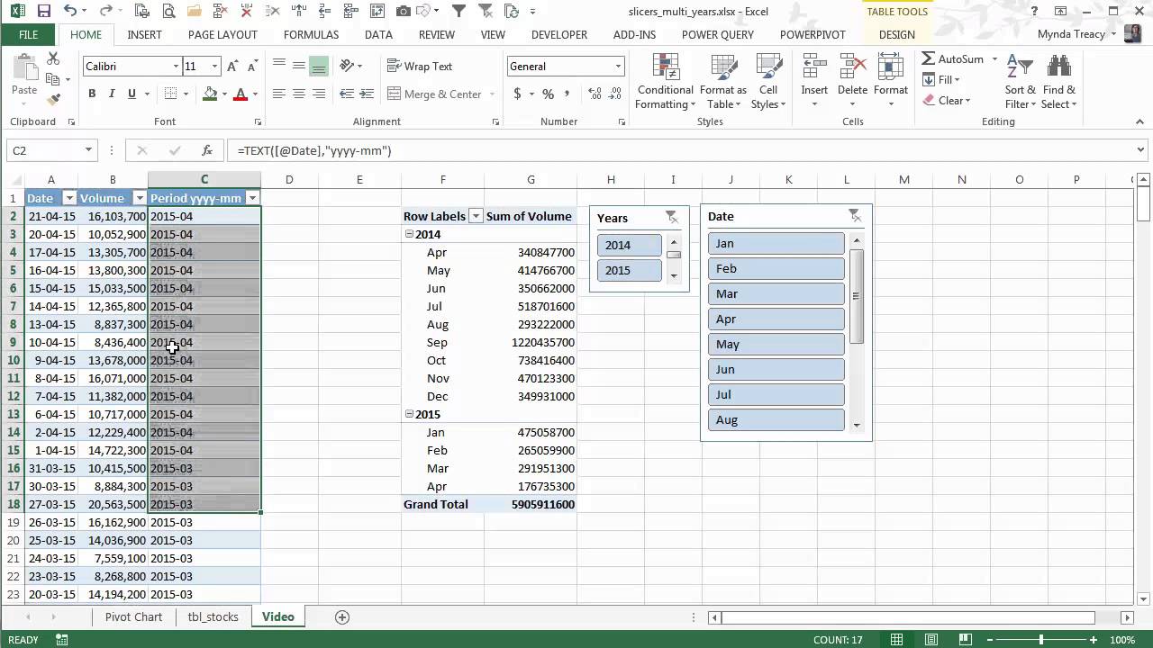
Slicers are particularly useful when working with PivotTables or PivotCharts. They provide an interactive and intuitive interface that allows you to slice and dice your data with ease. By simply clicking on the desired values in the Slicer, you can instantly filter your data and see the results in real-time.

To use a Slicer, first, make sure you have a PivotTable or PivotChart set up in your Excel sheet. Then, select the field or column that you want to use as the basis for filtering. Once you’ve selected the field, go to the “Insert” tab in the Excel ribbon and click on the “Slicer” button. A dialog box will appear, displaying all the available fields for you to choose from.

Select the desired field and click “OK”. Excel will insert a Slicer object into your sheet, displaying a list of unique values from the chosen field. You can customize the appearance of the Slicer by changing the size, color, and style to match the design of your worksheet.

To filter the data using the Slicer, simply click on the desired value(s) in the Slicer. Excel will instantly update the PivotTable or PivotChart to show only the data that matches your selection. You can choose multiple values to apply complex filters or use the “Clear Filter” button in the top-right corner of the Slicer to remove all filters.

Another great feature of Slicers is the ability to connect them to multiple PivotTables or PivotCharts. This allows you to control the filtering of data across different parts of your worksheet with a single Slicer. To connect a Slicer to another PivotTable or PivotChart, right-click on the Slicer, select “Report Connections”, and choose the desired objects to connect to. This way, any changes made to the Slicer will be automatically reflected in all connected objects.

Managing Slicers is also straightforward. You can resize, move, or delete a Slicer just like any other object in Excel. Right-click on the Slicer and select the desired action from the context menu. You can also format the Slicer by right-clicking on it and selecting “Slicer Settings”. In this settings window, you can change the caption, orientation, and other display options.

Customizing and managing Slicers

Once you have set up your Slicers in Excel, you have the option to customize and manage them to suit your specific needs. Customizing and managing Slicers allows you to fine-tune the appearance and behavior of the Slicers, giving you more control over how you filter and display data.

Here are some ways in which you can customize and manage Slicers in Excel:

1. Changing Slicer Styles: Excel provides various built-in styles for Slicers that you can choose from. These styles can help you match the Slicers with the overall look and feel of your Excel workbook. To change the Slicer style, simply select the Slicer, go to the Slicer Tools Design tab, and choose a different style from the available options.
2. Resizing and moving Slicers: You can resize and move Slicers to fit them better within your Excel worksheet. To resize a Slicer, select it and drag the sizing handles to adjust its dimensions. To move a Slicer, click and drag it to a new location on the worksheet.
3. Formatting Slicer elements: Excel allows you to format various elements of the Slicers, such as buttons, headers, and captions. You can change the font, font size, font color, background color, and other formatting options to make the Slicer more visually appealing or to match the formatting of other elements in your workbook.
4. Connecting multiple Slicers: If you have multiple Slicers in your Excel workbook, you can connect them to work together. For example, if you have a Slicer for region and another for product category, you can connect them so that selecting a region automatically updates the product category Slicer to show only the applicable categories for the selected region.
5. Managing Slicer settings: Excel provides various settings that you can use to customize the behavior of Slicers. For example, you can choose to hide the Slicer buttons or display them as a pop-up window. You can also choose to keep the Slicer visible even when there are no items selected, or automatically clear the selection when the workbook is closed.
6. Removing Slicers: If you no longer need a Slicer in your Excel workbook, you can easily remove it. To remove a Slicer, simply select it and press the Delete key or right-click on it and choose the “Remove Slicer” option.

By customizing and managing Slicers in Excel, you can enhance the functionality and aesthetics of your data filtering experience. Take advantage of the various customization options available to make your Slicers more visually appealing and user-friendly.

Conclusion

Now that you know how to use slicers to filter data in Excel, you can take your data analysis skills to the next level. Slicers not only make it easier to navigate and visualize your data, but they also provide a powerful tool for exploring and analyzing large datasets.

By utilizing slicers, you can instantly filter your data to focus on specific criteria, saving you time and effort. Whether you are tracking sales, analyzing trends, or managing inventory, slicers can help you uncover valuable insights and make informed decisions.

Remember to experiment with different slicer options and settings to tailor your data analysis experience to your specific needs. The more you practice using slicers, the more proficient you will become in extracting valuable information from your Excel spreadsheets.

So, go ahead and start applying the slicer functionality in Excel to supercharge your data analysis process and unlock the full potential of your datasets!

FAQs

Q: What are slicers in Excel?
A: Slicers in Excel are visual filters that allow you to easily filter data in a pivot table or pivot chart. They provide a user-friendly interface for filtering data by selecting specific values from a list.

Q: How do I insert a slicer in Excel?
A: To insert a slicer in Excel, first select the pivot table or pivot chart you want to filter. Then, go to the “PivotTable Tools” or “Chart Tools” tab in the Excel ribbon, depending on the type of object you have selected. In the “Insert Slicer” section, click on the “Slicer” button and choose the field(s) you want to use as filters. Click “OK” to insert the slicer.

Q: Can I use multiple slicers on the same Excel object?
A: Yes, you can use multiple slicers on the same Excel object. When you insert a slicer, you can choose multiple fields to use as filters. Each field will be represented by a separate slicer, allowing you to filter data based on different criteria simultaneously.

Q: Can I customize the appearance of the slicers in Excel?
A: Yes, you can customize the appearance of slicers in Excel. Right-click on a slicer and select “Slicer Settings” to open the options menu. From there, you can change the slicer’s style, size, position, and orientation. You can also apply a custom color scheme or use a slicer style from the gallery to match your Excel workbook’s overall theme.

Q: Can I connect multiple PivotTables or PivotCharts to the same slicer?
A: Yes, you can connect multiple PivotTables or PivotCharts to the same slicer. To do this, select a slicer and go to the “PivotTable Connections” or “Chart Connections” section in the “Slicer Tools” tab. Check the boxes corresponding to the objects you want to connect. This allows you to filter data across multiple objects simultaneously using the same slicer, ensuring consistency in your analysis.