
Connecting a slicer to multiple pivot tables with different data sources can greatly enhance the functionality and flexibility of your data analysis. Whether you’re a business analyst or a data enthusiast, being able to consolidate and analyze data from various sources is crucial to gaining valuable insights.
However, connecting a slicer to multiple pivot tables with different data sources may seem like a daunting task at first. Don’t worry, though – in this article, we’ll guide you through the process step by step, ensuring that you have a solid understanding of how to accomplish this task effortlessly. By the end of this article, you’ll have the knowledge and confidence to connect a slicer to multiple pivot tables, even when they have different data sources.
Inside This Article
- Overview
- Step 1: Add Data Tables for Each Pivot Table
- Step 2: Insert a Slicer
- Step 3: Connect the Slicer to the Pivot Tables
- Step 4: Customize Slicer Options
- Conclusion
- FAQs
Overview
Connecting a slicer to multiple pivot tables can be a game-changer when it comes to data analysis and presentation. It allows you to filter data across different data sources simultaneously, creating a more efficient workflow and saving you precious time. In this article, we will walk you through the steps to connect one slicer to multiple pivot tables with different data sources, empowering you to make meaningful insights from your data.
In order to connect a slicer to multiple pivot tables, you will need to follow a few simple steps. These steps include adding data tables for each pivot table, inserting a slicer, connecting the slicer to the pivot tables, and customizing the slicer options. By following these steps, you will be able to link multiple pivot tables to a single slicer, making your data analysis tasks even more powerful.
So, let’s dive into the details and learn how to connect a slicer to multiple pivot tables with different data sources. With this skill in your arsenal, you’ll be able to streamline your data analysis process and present your findings in a clear and comprehensive manner.
Step 1: Add Data Tables for Each Pivot Table
Before connecting a slicer to multiple pivot tables with different data sources, you need to ensure that you have the necessary data tables set up for each pivot table. This step helps establish the foundation for your analysis.
To add a data table for each pivot table, follow these steps:
- Identify the data sources: Determine the sources of data you will be using for each pivot table. This could be different tables within the same workbook or data from external sources such as databases or CSV files.
- Import or link the data: Import or link the data sources to your workbook by using the appropriate options in Excel. This ensures that the data is available for analysis and can be used in pivot tables.
- Create pivot tables: Once the data is imported or linked, create individual pivot tables for each data source. This can be done by selecting the data range and going to the “Insert” tab in Excel, then selecting “PivotTable” and choosing the desired location for the pivot table.
- Specify the data sources: While creating each pivot table, make sure to specify the respective data source for each table. This ensures that the correct data is used for analysis in each pivot table.
By following these steps, you will have separate data tables for each pivot table, allowing you to connect a slicer to multiple pivot tables with different data sources in the subsequent steps.
Step 2: Insert a Slicer
After adding the data tables for each pivot table, the next step is to insert a slicer to control the data displayed in all the pivot tables simultaneously. A slicer is a powerful tool in Excel that allows users to filter data easily and intuitively.
To insert a slicer, follow these steps:
- Select one of the pivot tables in which you want to insert the slicer. This will ensure that the slicer is connected to all the pivot tables.
- Click on the “Slicer” button in the “Insert” tab of the Excel ribbon. A dialog box will appear with a list of fields from the selected pivot table.
- Select the field that you want to use as the slicer. This field should be common among all the pivot tables, as the slicer will control the data displayed in all of them.
- Click on the “OK” button to insert the slicer. A slicer will appear on the worksheet, displaying the unique values of the selected field.
By default, the slicer will be created as a vertical list of buttons. You can resize and move the slicer to a convenient location on the worksheet. Furthermore, you can customize the slicer to suit your needs, such as changing the layout, style, and size.
Keep in mind that the slicer is now connected to the selected pivot table and will affect all the other pivot tables as well. Any filters applied to the slicer will instantly update the data displayed in all the connected pivot tables.
Continue to the next step to learn how to connect the slicer to the pivot tables.
Step 3: Connect the Slicer to the Pivot Tables
Now that we have added the necessary data tables and inserted the slicer, it’s time to connect the slicer to the pivot tables. This step ensures that selecting a value in the slicer will filter the data in all the pivot tables simultaneously.
To connect the slicer to the pivot tables, follow these steps:
- Click on the slicer to activate it.
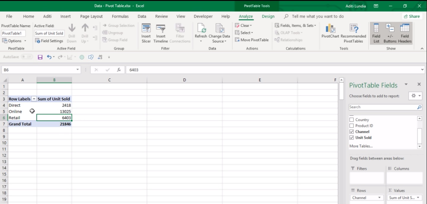
- In the PivotTable Tools tab, navigate to the Analyze tab.
- In the Filter group, click on the “Insert Slicer Connection” button.
- A dialog box will appear, showing all the pivot tables in your workbook. Select the pivot tables that you want to connect to the slicer by checking the corresponding checkboxes.
- Click on the “OK” button.
Now, the slicer is connected to the selected pivot tables. Any selection made in the slicer will automatically update the data displayed in the connected pivot tables.
It’s important to note that when connecting the slicer to multiple pivot tables, any pivot table with a common field will be filtered based on the slicer selection. This allows for easy comparison and analysis across different data sources.
Additionally, if you have multiple slicers in your workbook, you can repeat this step to connect them to the desired pivot tables, further enhancing the interactivity and functionality of your reports.
Once connected, feel free to explore different slicer selections and watch as the pivot tables dynamically update to reflect the chosen values.
Connecting the slicer to multiple pivot tables provides a seamless way to analyze and visualize data from different sources, enabling you to gain valuable insights and make informed decisions.
Now that you have successfully connected the slicer to the pivot tables, let’s move on to the next step to customize the slicer options.
Step 4: Customize Slicer Options
Once you have connected the slicer to your pivot tables and added the necessary data tables, you can further customize the slicer options to enhance the user experience. Here are a few ways to customize your slicer:
1. Change Slicer Style: You have the option to change the appearance of the slicer by selecting a different style. Simply right-click on the slicer and choose “Slicer Styles” from the context menu. Experiment with different styles until you find the one that best matches your data visualization needs.
2. Format Slicer Buttons: You can modify the format of the buttons within the slicer to make them stand out or match your overall design scheme. Select the slicer, and in the “Slicer Tools” contextual tab, click on the “Options” tab. From here, you can change the button size, font style, color, and other formatting options.
3. Enable Multi-Select: By default, slicers allow users to select only one item at a time. However, you can enable multi-select to give users the flexibility to choose multiple items simultaneously. To do this, right-click on the slicer and select “Slicer Settings.” In the settings dialog box, check the “Allow multiple selections” option.
4. Control Slicer Display: You can control how the slicer is displayed to optimize the user experience. Right-click on the slicer and select “Slicer Settings.” In the settings dialog box, you can choose to show items with no data, hide items with no data, or hide the slicer if there is no data. This helps to ensure that only relevant and meaningful slicer options are displayed.
5. Customize Slicer Caption and Size: If you want to provide additional information or instructions to your users, you can customize the slicer caption. Simply select the slicer and in the “Slicer Tools” contextual tab, click on “Options.” Here, you can enter a descriptive caption to guide users in manipulating the slicer. Additionally, you can resize the slicer by dragging its edges to fit your desired dimensions.
By customizing the slicer options, you can tailor the visual representation of your data to suit your specific needs. This allows users to have a seamless and intuitive experience while efficiently navigating through multiple pivot tables with different data sources.
Conclusion
Connecting a slicer to multiple pivot tables with different data sources can be a powerful way to streamline your data analysis workflow. By following the steps outlined in this article, you can easily link a slicer to multiple pivot tables and create dynamic reports that allow for seamless filtering of data.
Through the use of slicers, you can enhance the interactivity and usability of your pivot tables, making it easier to analyze and present data effectively. Whether you are working on complex financial analysis, sales reports, or any other data-driven task, connecting a slicer to multiple pivot tables will save you time and effort.
Remember to ensure that your data sources are compatible and properly organized, and experiment with various filtering options to gain deeper insights into your data. With this knowledge, you can unlock the full potential of your pivot tables and make well-informed decisions based on your analysis.
So, why wait? Start connecting slicers to multiple pivot tables today and take your data analysis to the next level!
FAQs
Q: Can I connect a slicer to multiple pivot tables with different data sources?
Absolutely! One of the great features of slicers in Excel is the ability to connect them to multiple pivot tables, even if those tables have different data sources. This allows you to control the filtering of data in multiple pivot tables simultaneously, making data analysis and reporting much more efficient.
Q: How do I connect a slicer to multiple pivot tables with different data sources?
To connect a slicer to multiple pivot tables with different data sources, follow these steps:
- Create a slicer that is connected to one of the pivot tables.
- Right-click on the slicer and select “Report Connections”.
- In the Report Connections dialog box, check the boxes next to the pivot tables you want the slicer to affect.
- Click OK to apply the changes.
Now, when you use the slicer to filter data in one pivot table, it will automatically update the other connected pivot tables as well.
Q: Can I connect a slicer to pivot tables on different worksheets or workbooks?
Yes, you can connect a slicer to pivot tables on different worksheets or workbooks. The process is similar to connecting a slicer to pivot tables with different data sources. Follow the steps mentioned above, and instead of selecting pivot tables within the same worksheet, you can select pivot tables from different worksheets or even different workbooks.
Q: What happens if I disconnect a slicer from a pivot table?
If you disconnect a slicer from a pivot table, the slicer will no longer control the filtering of data in that pivot table. However, the slicer will still be available for use with other connected pivot tables. Disconnecting a slicer can be useful when you want to focus the filtering on specific pivot tables or when you want to change the connection between slicer and pivot table.
Q: Can I customize the appearance of slicers connected to multiple pivot tables?
Yes, you can customize the appearance of slicers connected to multiple pivot tables. Right-click on the slicer and select “Slicer Styles” to choose from a variety of pre-defined styles. You can also modify the slicer settings, such as the orientation, size, and button captions, by right-clicking on the slicer and selecting “Slicer Settings”. Customizing the appearance of slicers can help you enhance the visual appeal and usability of your dashboards and reports.
Q: Is it possible to connect a slicer to pivot tables in different versions of Excel?
Yes, it is possible to connect a slicer to pivot tables in different versions of Excel. Slicers were introduced in Excel 2010, so as long as you are using a version that includes slicer functionality, you should be able to connect them to your pivot tables. However, keep in mind that some older versions of Excel may have limited slicer features compared to newer versions.