
If you want to make your data more visually appealing and easier to interpret, one effective technique is to use solid fill red data bars. These bars provide a clear visual representation of data values, allowing you to quickly identify high and low points. Whether you’re working with spreadsheets or analyzing data in a presentation, adding solid fill red data bars can greatly enhance the overall impact and clarity of your information. In this article, we will guide you step-by-step on how to add solid fill red data bars to your data sets, regardless of the program you are using. With the right knowledge and a few simple steps, you’ll be able to create visually impactful data displays that will captivate your audience and make your information stand out.
Inside This Article
- Step 1: Open the Spreadsheet
- Step 2: Select the Data Range
- Step 3: Click on “Conditional Formatting”
- Step 4: Choose “New Rule”
- Step 5: Select “Format only cells that contain”
- Step 6: Specify the Format Style
- Step 7: Set the Fill Color to Red
- Step 8: Apply the Data Bars to the Selected Range
- Conclusion
- FAQs
Step 1: Open the Spreadsheet
Before you can add solid fill red data bars to your spreadsheet, you need to open the spreadsheet file that contains the data you want to format. Whether you’re using Microsoft Excel, Google Sheets, or any other spreadsheet software, the first step is to launch the program and open the desired file.
Once you have the spreadsheet open, make sure you locate the specific sheet or tab that contains the data you want to format. If your spreadsheet has multiple sheets, you may need to navigate to the correct one by clicking on the respective tab at the bottom of the program window.
It’s important to ensure that the spreadsheet is editable. If the file is read-only or if you don’t have the necessary permissions to make changes, you won’t be able to add solid fill red data bars or apply any other formatting options.
Additionally, make sure that the data you want to format is arranged in columns or rows within the sheet. The data bars are typically applied to a range of cells that represent a specific data set. By opening the spreadsheet and navigating to the appropriate sheet, you’re ready to move on to the next step of adding solid fill red data bars.
Step 2: Select the Data Range
After opening the spreadsheet in your preferred application, the next step is to select the specific data range that you want to apply the solid fill red data bars to. This range can consist of a single column of data, multiple columns, or even a range that includes both columns and rows. The data range should be a contiguous block of cells, meaning they are adjacent to each other without any gaps or breaks.
To select the data range, simply click and hold the left mouse button on the first cell of the range, then drag the cursor to the last cell of the range. Alternatively, you can click on the first cell, then hold the Shift key and click on the last cell to select the entire range in one go.
If you have a large amount of data and it’s difficult to scroll to the last cell, you can speed up the selection process by using keyboard shortcuts. For example, you can select the first cell of the range, press and hold the Shift key, then use the arrow keys to extend the selection to the desired cells. This method is particularly useful when working with long columns or wide rows of data.
Ensure that you have selected all the necessary cells within the desired range before proceeding to the next step. Double-checking your selection will help avoid applying the solid fill red data bars to unintended cells.
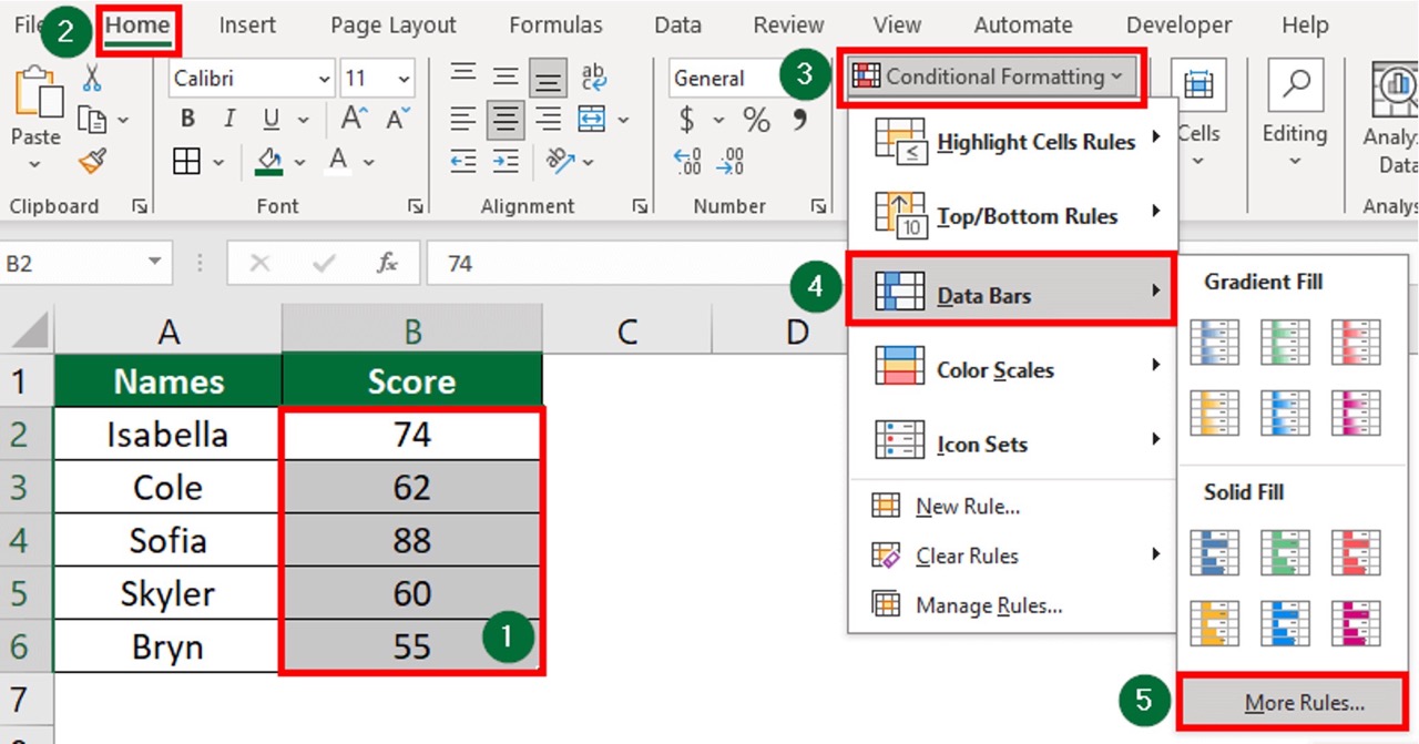
Step 3: Click on “Conditional Formatting”
Conditional Formatting is a powerful feature in spreadsheet programs that allows you to apply different formatting styles to cells based on specified criteria. It is a handy tool when you want to highlight certain data or add visual cues to your spreadsheet. To start using Conditional Formatting, follow the steps below:
1. Once you have your spreadsheet open, navigate to the toolbar at the top of the program.
2. Look for the “Format” or “Home” tab, depending on the spreadsheet program you are using. Click on it to reveal a drop-down menu.
3. From the drop-down menu, locate and click on the option called “Conditional Formatting.” This will open a sidebar or dialog box with various formatting options.
4. The Conditional Formatting feature allows you to define rules, or conditions, for applying specific formatting styles. These rules can be based on values, formulas, or even custom criteria you set.
5. Depending on your spreadsheet program, you may have different options for conditional formatting. Common options include highlighting cells that contain specific text, values greater than or less than a certain number, or based on the contents of other cells.
6. Once you have selected your desired conditional formatting rule, you may have additional options to fine-tune the formatting. These options can include choosing font styles, text color, background color, and more.
7. After setting up your desired conditional formatting rule and formatting options, click on the “Apply” or “OK” button to apply the rule to your selected range of cells.
By clicking on “Conditional Formatting,” you open a world of possibilities for customizing and highlighting your spreadsheets. This feature is particularly useful when dealing with large datasets or when you want to draw attention to specific data points. Take advantage of it to make your spreadsheets more visually appealing and easier to read.
Step 4: Choose “New Rule”
Once you have selected the data range you want to apply the solid fill red data bars to, it’s time to move on to the next step. In this step, you will choose the “New Rule” option to set up the specific rule for the data bars.
To choose “New Rule,” you will need to follow these steps:
- Click on the “Conditional Formatting” button located in the “Home” tab of the Excel ribbon. This will open a drop-down menu with various formatting options.
- In the drop-down menu, select “New Rule.” This will open a dialog box with different rule options to choose from.
Choosing “New Rule” allows you to specify the conditions under which the solid fill red data bars should be applied to your selected data range. This step is important as it determines the criteria for displaying the data bars.
By selecting “New Rule,” you gain access to a wide range of formatting options. These options include highlighting cells that are above or below a certain threshold, containing specific text, or meeting other statistical conditions. The flexibility offered by the “New Rule” feature enables you to create custom rules that suit your specific needs.
For example, you can choose “New Rule” to specify that the data bars should only be applied to the cells that contain numbers greater than a certain value. Alternatively, you can set up a rule that highlights cells with specific text or formula results. The “New Rule” option gives you the power to tailor the appearance of the data bars based on your desired conditions.
Once you have chosen the “New Rule” option, you can proceed to the next step, where you will specify the format style for the data bars. This format style will determine the visual appearance of the solid fill red data bars when applied to your selected data range.
Step 5: Select “Format only cells that contain”
Once you have opened the spreadsheet and selected the desired range of cells, it’s time to move on to the next step: selecting the option to format only the cells that contain specific criteria. This feature allows you to apply the solid fill red data bars to cells that meet certain conditions, making it easy to visually identify data trends or patterns.
To achieve this, locate the “Conditional Formatting” button in the toolbar of your spreadsheet application. It is usually located under the Home or Format tab, depending on the software you are using. Click on this button to reveal a dropdown menu of formatting options.
From the dropdown menu, select the “Format only cells that contain” option. This will open a dialog box that provides various criteria to choose from. These criteria allow you to determine which cells will be highlighted with the solid fill red data bars.
In this step, you have the flexibility to select the criteria that best suit your needs. You can choose from options such as numbers that are greater than or less than a certain value, cells that contain specific text or dates, or even create custom formulas to define your own criteria.
By selecting “Format only cells that contain”, you are empowering yourself with the ability to visually emphasize important data points. This step allows you to go beyond mere data entry and analysis, turning your spreadsheet into a powerful tool for data visualization.
Once you have chosen your desired criteria, you are ready to proceed to the next step, where you will specify the format style for the solid fill red data bars. This is the final customization step before applying the formatting to the selected cell range.
Step 6: Specify the Format Style
Once you have chosen “New Rule” in the previous step, a dialog box will appear with various options for formatting the data bars. This is where you can specify the format style that you want for your solid fill red data bars.
In the “Format Style” section of the dialog box, you will see a drop-down menu with different options. The most common format style is “Gradient Fill,” which creates a gradual transition of colors along the length of the data bars. However, since we want solid fill red data bars, we will select the “Solid Fill” option.
By selecting the “Solid Fill” option, you are instructing the spreadsheet program to fill the data bars with a single color from start to end. In this case, the color will be red, as specified in the previous steps.
In addition to selecting the format style, you can also specify other options such as the minimum and maximum values for the data bars, as well as the type of data bars (such as positive and negative bars). However, these options are not necessary for creating solid fill red data bars, so you can leave them at their default values.
Once you have specified the format style and any other desired options, click on the “OK” button to apply the changes and close the dialog box.
Step 7: Set the Fill Color to Red
Once you have selected the data range and specified the format style for your data bars, the next step is to set the fill color to red. This will give your data bars a solid fill color of red, making them visually impactful and easy to interpret.
To set the fill color, follow these simple steps:
- Select the data range that you want to apply the solid fill red data bars to.
- Click on the “Conditional Formatting” option in the toolbar.
- From the dropdown menu, select “New Rule”.
- In the “New Formatting Rule” dialog box, choose the option “Format only cells that contain”.
- Below that, you will find the “Format Style” section. Click on the “Fill” tab.
- Choose the red color from the available color options.
- Adjust the transparency or opacity of the fill color if desired.
- Click “OK” to apply the fill color to the selected data range.
By setting the fill color to red, you can easily identify and distinguish the values that fall within the data bars. This visual representation helps you quickly analyze the relative values and trends in your data.
Step 8: Apply the Data Bars to the Selected Range
Now that you have set the format style and fill color for the data bars, it’s time to apply them to the selected range in your spreadsheet. Here’s how you can do it:
1. With the data range still selected, go back to the “Conditional Formatting” menu.
2. Choose the “Data Bars” option. This will display a drop-down menu with different data bar styles.
3. Select the “Solid Fill Red” data bar style from the drop-down menu. This will apply the solid red color fill to the data bars.
4. Once you have selected the desired data bar style, click on “Apply” or “OK” to confirm. The data bars will now be applied to the selected range of cells in your spreadsheet.
5. Take a moment to review the applied data bars and make any necessary adjustments. You can resize the width of the data bars or modify the formatting options by going back to the “Conditional Formatting” menu.
By applying the data bars to the selected range, you can now visually highlight the relative values of the cells in your spreadsheet. This can be particularly useful for analyzing trends, comparing data, or identifying outliers at a glance.
Remember, the data bars can be customized further to suit your preferences. You can experiment with different colors, gradient fills, or even customize the data bars based on your specific criteria or thresholds.
Now that you have successfully applied the data bars with a solid red fill to the selected range, you can take full advantage of this visual tool to enhance your data analysis and presentation!
Conclusion
In conclusion, adding solid fill red data bars to your cell phone is a great way to enhance its visual appeal and make it stand out from the crowd. By implementing this customization feature, you can give your phone a unique and personalized touch that reflects your style and personality.
The process of adding solid fill red data bars may vary depending on the make and model of your cell phone, but the general steps involve accessing the settings or customization options, selecting the data bar feature, and choosing the red color from the available palette. Once applied, you will be able to enjoy a visually stunning and eye-catching data bar on your phone’s screen.
Whether you want to add solid fill red data bars for professional or personal reasons, this customization feature can provide a fresh and vibrant look to your phone’s display. So why wait? Give your cell phone a bold and striking appearance today by adding solid fill red data bars!
FAQs
1. How do I add solid fill red data bars to my cells?
Adding solid fill red data bars to cells is a simple process. First, select the range of cells where you want to apply the data bars. Then, go to the “Home” tab in Microsoft Excel and click on the “Conditional Formatting” button. From the dropdown menu, choose “Data Bars” and then select the desired type of data bar. In this case, choose the solid fill red data bar. The selected cells will now have red data bars indicating their values.
2. Can I customize the solid fill red data bars?
Yes, you can customize the solid fill red data bars to suit your preferences or your specific needs. After applying the solid fill red data bars to the selected cells, right-click on any of the data bars and choose “Conditional Formatting” from the dropdown menu. This will open the Conditional Formatting dialog box. Here, you can adjust various parameters such as the minimum and maximum values to which the data bars are applied, the color of the data bars, and the style, among other options. Once you have made the desired changes, click “OK” to apply the customization to the data bars.
3. Can I apply solid fill red data bars to specific cells based on a certain condition?
Certainly! Microsoft Excel allows you to apply solid fill red data bars to specific cells based on certain conditions. To do this, you will need to use conditional formatting rules. Select the range of cells you want to apply the data bars to, go to the “Home” tab, click on “Conditional Formatting,” and choose “New Rule” from the dropdown menu. In the New Formatting Rule dialog box, select “Use a formula to determine which cells to format” and enter the formula that defines the condition for the solid fill red data bars. For example, if you want to apply the data bars to cells that have a value greater than a specific threshold, the formula could be something like “=A1>50”. Once you have entered the formula, choose the format for the data bars, including the solid fill red option, and click “OK” to apply the rule.
4. Can I remove solid fill red data bars from specific cells?
Absolutely! If you want to remove the solid fill red data bars from specific cells, you can do so by following these steps. Select the range of cells from which you want to remove the data bars. Then, go to the “Home” tab, click on “Conditional Formatting,” and choose “Clear Rules” from the dropdown menu. From the submenu, select “Clear Rules from Selected Cells” or “Clear Rules from Entire Sheet,” depending on your specific needs. This will remove the solid fill red data bars from the selected cells, leaving them with their original formatting.
5. Are solid fill red data bars available in other spreadsheet programs?
Solid fill red data bars are specific to Microsoft Excel and may not be available in other spreadsheet programs. However, other programs may offer similar features or ways to visually represent data. If you are using a different spreadsheet program, consult its documentation or help resources to explore the available options for visually highlighting data in a similar manner.