
If you’re a frequent user of Microsoft Excel, chances are you’ve come across the powerful tool known as the Pivot Table. It’s a feature that enables users to summarize and analyze large amounts of data with just a few clicks. But have you ever wondered where the data for a Pivot Table actually comes from? Understanding the data source is crucial for ensuring the accuracy and reliability of your analysis. In this article, we’ll explore how to see the data source for a Pivot Table in Excel. Whether you’re a seasoned Excel user or just getting started, this knowledge will help you harness the full potential of Pivot Tables and make better-informed decisions based on your data. So, let’s dive in and discover the secrets behind the data source of a Pivot Table.
Inside This Article
- Overview
- Step 1: Open the Pivot Table
- Step 2: Navigate to the Field List
- Step 3: View the Data Source
- Step 4: Modify the Data Source if Needed
- Step 5: Refresh the Pivot Table Data
- Step 6: Verify the Data Source of the Pivot Table
- Conclusion
- FAQs
Overview
When working with a pivot table, it is important to know the source of the data being used. By understanding the data source, you can ensure that the information displayed in the pivot table is accurate and up-to-date. In this article, we will guide you through the steps to see the data source for a pivot table and how to modify it if needed.
Pivot tables are a powerful tool in data analysis, allowing you to summarize and analyze large amounts of data. They provide a dynamic and interactive way to organize and analyze data, making it easier to identify trends, patterns, and outliers. However, to fully leverage the power of pivot tables, you need to have a clear understanding of the source data.
By default, when you create a pivot table in Excel, it uses the data from a specific range or table in your worksheet as the source. This range of data is what determines the values, rows, and columns in your pivot table. It is important to be able to see and verify this data source to ensure the accuracy of your analysis.
The process of viewing the data source for a pivot table is straightforward and can be done in a few simple steps. Let’s dive in and explore how to view the data source for a pivot table in Excel.
Step 1: Open the Pivot Table
Opening the pivot table is the first step to viewing its data source. A pivot table is a powerful data analysis tool that allows you to summarize and analyze large data sets. Before you can see the data source, you need to have a pivot table created in the first place.
To open the pivot table, you will need a spreadsheet program like Microsoft Excel or Google Sheets. Open the program and navigate to the workbook that contains the pivot table you want to view.
Once you have the workbook open, locate the sheet that contains the pivot table. This is usually indicated by a tab at the bottom of the program window. Click on the tab to switch to the sheet where the pivot table is located.
With the sheet containing the pivot table active, locate the pivot table itself. The pivot table is a visually organized representation of your data that allows you to perform various calculations and analysis. It typically consists of rows, columns, and values.
Click on any part of the pivot table to select it. This will activate the pivot table and allow you to interact with it. You will now be able to view and modify the pivot table settings.
By following these steps, you have successfully opened the pivot table and are now ready to proceed to the next step of viewing the data source!
Step 2: Navigate to the Field List
Once you have opened your Pivot Table, the next step is to navigate to the Field List. The Field List is a panel that contains all the available fields or columns from your data source. It allows you to select the fields you want to analyze and drag them into different areas of the Pivot Table.
To access the Field List, you need to look for the Field List icon or button, which is usually located on the right side of the Pivot Table interface. It is represented by a small grid or a button labeled “Field List”. Click on this icon or button to open the Field List panel.
Upon opening the Field List, you will see a list of fields from your data source organized into different categories. These categories are usually based on the structure of your data, such as columns, rows, values, and filters. Each category represents a specific role within the Pivot Table.
Take a moment to explore and familiarize yourself with the Field List panel. You can scroll through the list of fields and expand or collapse the categories to find the specific fields you want to include in your Pivot Table.
Once you have identified the desired fields, you can simply drag and drop them into the corresponding areas of the Pivot Table. For instance, if you want to analyze sales data by product category, you can drag the “Product Category” field into the Row Labels area. Similarly, if you want to calculate the total sales amount, you can drag the “Sales Amount” field into the Values area.
Remember that you can always customize the Pivot Table by adding or removing fields as needed. The Field List provides the flexibility to modify your analysis based on the specific insights you want to uncover.
Now that you have successfully navigated to the Field List and selected the fields for your analysis, it’s time to move on to the next step – viewing the data source of the Pivot Table.
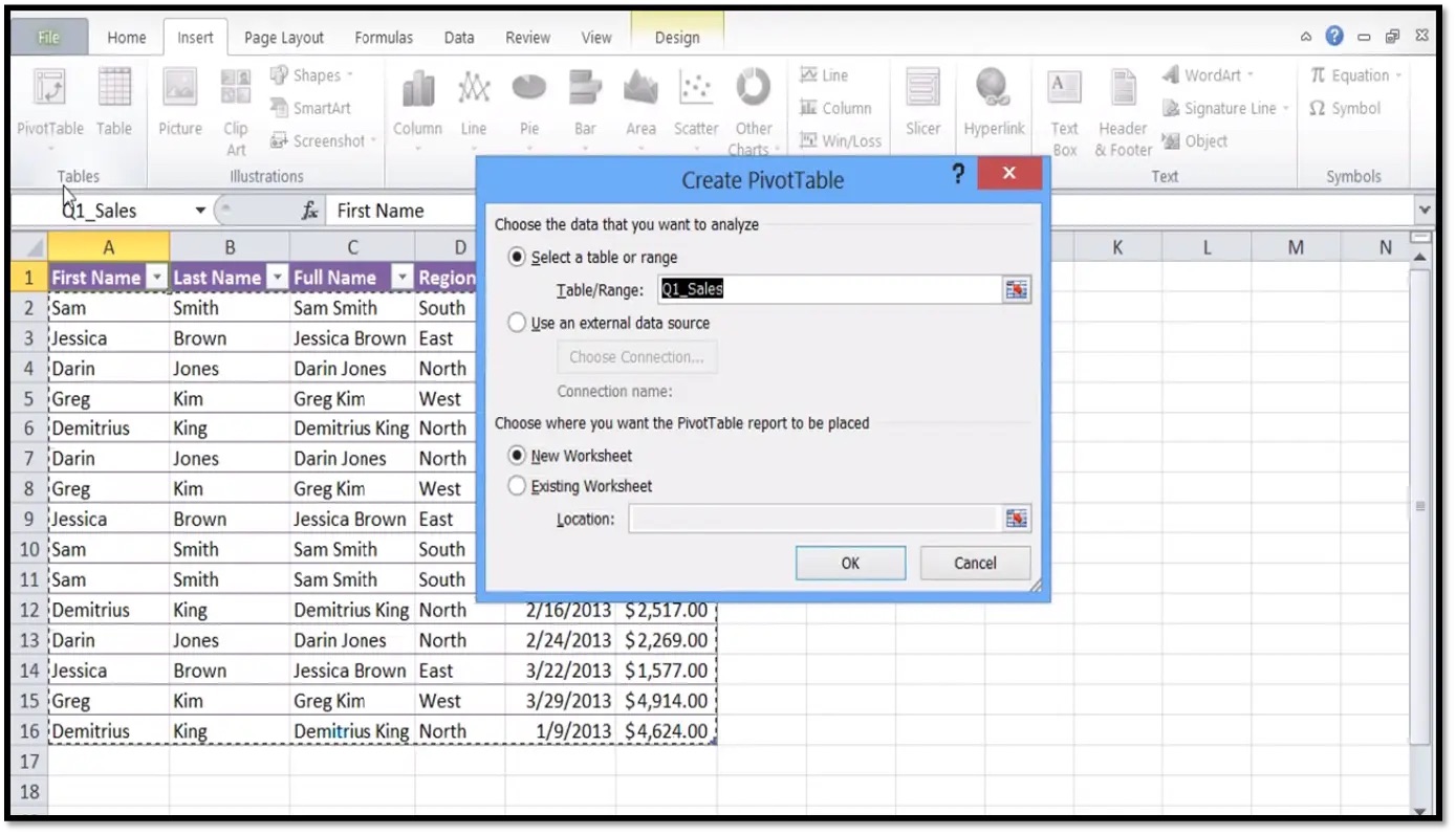
Step 3: View the Data Source
In order to see the data source for a pivot table, you’ll need to follow a few simple steps. Once you have opened the pivot table and selected the specific table or range that you want to analyze, you can proceed to view the data source.
1. In your Excel worksheet, click on the pivot table to activate it. This will display the PivotTable Tools contextual tab in the Excel ribbon.
2. Within the PivotTable Tools tab, navigate to the “Analyze” tab and locate the “Data” group.
3. Click on the “Change Data Source” button in the “Data” group. This will open a dialog box that allows you to view and modify the data source for your pivot table.
4. The dialog box will display the current data source for your pivot table. It will show the table or range that you selected when creating the pivot table.
5. You can also click on the “Browse” button to locate and select a different data source for your pivot table if needed.
6. Once you have viewed the data source and made any necessary modifications, click on the “OK” button to save your changes and close the dialog box.
By following these steps, you will be able to easily view the data source for your pivot table. This information is useful for understanding the underlying data that is being analyzed and can be helpful if you need to make any changes to the data source or refresh the pivot table data.
Step 4: Modify the Data Source if Needed
After viewing the data source for your pivot table, you may realize that it needs some modifications. Whether it’s adding or removing data, or even changing the source altogether, Excel provides you with the flexibility to make these adjustments.
To modify the data source of your pivot table, follow these steps:
- Click on the Pivot Table to select it.
- In the PivotTable Tools tab, click on the Analyze or Options tab (depending on your Excel version).
- Click on the Change Data Source button.
- In the Change PivotTable Data Source dialog box, you can modify the range or table selection for your data source. You can also add or remove columns or rows from the data.
- Click on OK to apply the changes.
By modifying the data source, you can customize the information included in your pivot table to meet your specific needs. This can be particularly useful if you want to analyze different sections of your data or if you have made updates to the original data set.
It’s worth noting that modifying the data source could have an impact on the layout and structure of your pivot table. Therefore, it’s essential to review and adjust the pivot table layout if necessary.
Once you have made the required modifications to the data source, you can proceed to the next step to refresh the pivot table data.
Step 5: Refresh the Pivot Table Data
Once you have created a pivot table and made changes to the source data, you need to refresh the pivot table to ensure that the data is up to date. Refreshing the pivot table will recalculate the summarized data based on the updated source data. Here’s how you can refresh the pivot table data:
1. Click on any cell within the pivot table to activate it.
2. Go to the “Analyse” or “Options” tab in the Excel Ribbon, depending on your version of Microsoft Excel.
3. Look for the “Refresh” button or option. It is usually located in the “Data” group.
4. Click on the “Refresh” button to refresh the pivot table.
5. Alternatively, you can right-click on the pivot table and select “Refresh” from the context menu.
6. Once you click on the “Refresh” button, Excel will update the pivot table with the latest data from the source.
7. If there are any changes in the source data, such as new records or updated values, the pivot table will reflect those changes after refreshing.
8. You can also automate the refreshing process by selecting the “Refresh data when opening the file” option. This way, the pivot table will be automatically refreshed every time you open the Excel file.
By regularly refreshing the pivot table data, you can ensure that your analysis is based on the most current information. This is particularly useful when working with dynamic datasets or when collaborating with others.
Next, let’s move on to the final step to verify the data source of the pivot table.
Step 6: Verify the Data Source of the Pivot Table
After setting up a pivot table and connecting it to a data source, it’s important to verify the data source to ensure the accuracy and reliability of your analysis. With just a few steps, you can easily confirm the data source of your pivot table and make any necessary adjustments if needed.
The process of verifying the data source of a pivot table may vary slightly depending on the spreadsheet software you are using. However, the general steps remain consistent across different platforms. In this guide, we will cover the steps for verifying the data source in Microsoft Excel, one of the most widely used spreadsheet programs.
To begin, select the pivot table that you want to verify. This can be done by clicking anywhere inside the pivot table or by selecting the cell range that contains the pivot table data.
Next, navigate to the “Analyze” or “Options” tab in the Excel ribbon, depending on your version of Excel. Look for the “Change Data Source” or “PivotTable Data Source” button, and click on it. This will open a dialog box that displays the current data source of the pivot table.
In the dialog box, you will see a table range or a named range that represents the data source of the pivot table. Take a moment to review this information and make sure it matches the intended data range. If you notice any discrepancies, you can adjust the data source by selecting the correct range using the table range selector or manually typing in the range.
After verifying and adjusting the data source, click the “OK” button to save your changes. This will update the pivot table and ensure it reflects the correct data range.
At this point, it is crucial to refresh the pivot table to ensure the changes to the data source are applied. To refresh the pivot table, right-click on the pivot table and select the “Refresh” option. Alternatively, you can go to the “Analyze” or “Options” tab and click on the “Refresh” button.
Finally, it is essential to double-check the data source of the pivot table to confirm that everything is in order. Repeat Step 2 by navigating to the “Change Data Source” or “PivotTable Data Source” button and verify that the displayed data source matches your intended range.
By following these steps, you can easily verify and ensure the accuracy of the data source used in your pivot table. This not only gives you confidence in the reliability of your analysis but also helps you make informed decisions based on the correct data.
Remember, maintaining accurate and up-to-date data sources is crucial for accurate business insights and improved decision-making. Take the time to verify your pivot table’s data source regularly and make any necessary adjustments to ensure the integrity of your analysis.
Conclusion
In conclusion, understanding how to see the data source for a pivot table is essential for effectively analyzing and manipulating data in Excel. By following the steps outlined in this article, you can easily view and modify the data source of your pivot table, allowing you to make updates and changes as needed.
Remember to start by selecting the pivot table and going to the “Analyze” or “Options” tab, depending on your version of Excel. From there, click on the “Change Data Source” button and make the necessary adjustments to the range of data you want to include in your pivot table.
By having a clear understanding of the data source for your pivot table, you can ensure accurate and meaningful analysis, leading to better decision-making. So, take the time to explore and master this feature, and unlock the full potential of pivot tables in Excel.
FAQs
1. How do I see the data source for a pivot table?
2. Can I change the data source for a pivot table?
3. What happens if I delete or move the data source of a pivot table?
4. Is it possible to add multiple data sources to a single pivot table?
5. Can I create a pivot table from an external data source?