How To Define Maximum Data Bars Value In Excel

Excel’s data bars feature is a powerful tool for visualizing data in a worksheet. Data bars provide a simple and effective way to display the relative value of a cell compared to other cells in the range. By default, Excel automatically determines the maximum value for the data bars based on the highest value in the selected range. However, there may be scenarios where you want to define a specific maximum value for the data bars. In this article, we will explore different methods to define the maximum data bars value in Excel.

Method 1: Adjusting the Maximum Value Manually

The simplest way to define the maximum data bars value is by manually adjusting it in Excel. Here’s how you can do it:

Select the range of cells that you want to apply data bars to.
Go to the “Home” tab and click on the “Conditional Formatting” dropdown.
Select “Data Bars” and then click on “More Rules” at the bottom of the dropdown.
In the “New Formatting Rule” dialog box, select “Number” as the type.
Enter the desired maximum value in the “Maximum” field.
Click “OK” to apply the changes.

This method allows you to manually set the maximum value for the data bars, giving you full control over the scale of the bar lengths.

Method 2: Using a Formula to Set the Maximum Value

If you want the maximum value for the data bars to be dynamic and based on a specific formula, you can use a formula to define it. Here’s how:

Select the range of cells that you want to apply data bars to.
Go to the “Home” tab and click on the “Conditional Formatting” dropdown.
Select “Data Bars” and then click on “More Rules” at the bottom of the dropdown.
In the “New Formatting Rule” dialog box, select “Formula” as the type.
Enter the formula that calculates the maximum value in the “Value” field.
Click “OK” to apply the changes.

This method allows you to define the maximum value for the data bars based on a formula, allowing for greater flexibility and customization.

Method 3: Using Conditional Formatting to Set the Maximum Value

Excel’s conditional formatting feature can also be used to define the maximum value for data bars. Here’s how:

Select the range of cells that you want to apply data bars to.
Go to the “Home” tab and click on the “Conditional Formatting” dropdown.
Select “New Rule” to open the “New Formatting Rule” dialog box.
Select the option “Format only cells that contain” and choose “Greater Than or Equal To” as the condition.
Enter the desired maximum value in the “Value” field.
Click “OK” to apply the changes.

This method allows you to set the maximum value for the data bars using conditional formatting rules, providing more advanced control over the appearance of the bars.

Method 4: Creating a Custom Data Bar Format with Maximum Value

If you want to have complete control over the appearance of the data bars, including the maximum value, you can create a custom data bar format. Here’s how:

Select the range of cells that you want to apply data bars to.
Go to the “Home” tab and click on the “Conditional Formatting” dropdown.
Select “New Rule” to open the “New Formatting Rule” dialog box.
Select “Use a formula to determine which cells to format” as the rule type.
Enter the formula that evaluates to TRUE for the cells you want to apply the data bars to.
Click on the “Format” button to open the “Format Cells” dialog box.
Go to the “Fill” tab and select the desired fill color for the data bars.
Adjust the “Maximum” value in the data bar settings to define the maximum value for the bars.
Click “OK” to apply the changes.

This method gives you complete control over the data bar format, including the maximum value, allowing you to create custom visualizations tailored to your specific needs.

Steps to Define Maximum Data Bars Value

Excel’s data bars feature is a great way to visualize the values in your spreadsheet. By using data bars, you can quickly identify the high and low values in a range of cells. However, sometimes the default maximum value for data bars may not accurately represent the range of data you want to display. In this article, we will guide you through the steps to define the maximum data bars value in Excel.

There are several ways you can define the maximum value for data bars in Excel. Let’s explore each method:

Adjusting the Maximum Value Manually: One way to set the maximum data bars value is to adjust it manually. You can do this by selecting the cells with data bars, going to the “Conditional Formatting” menu, selecting “Manage Rules,” and editing the rule for data bars. From there, you can manually specify the maximum value for the data bars.
Using a Formula to Set the Maximum Value: Another method is to use a formula to calculate and set the maximum value for the data bars. For example, you can use the MAX function to determine the maximum value in a range of cells, and then use that result as the maximum value for the data bars.
Using Conditional Formatting to Set the Maximum Value: Excel’s conditional formatting feature can also be used to set the maximum value for data bars. By creating a conditional formatting rule based on a formula, you can dynamically determine the maximum value for the data bars. This allows the maximum value to update automatically as your data changes.
Creating a Custom Data Bar Format with Maximum Value: If none of the above methods suit your needs, you can also create a custom data bar format with a specific maximum value. This involves creating a new data bar format and manually specifying the maximum value, as well as the appearance of the data bar.

By following these steps, you can easily define the maximum data bars value in Excel. Whether you prefer to adjust it manually, use a formula, or leverage conditional formatting, Excel provides flexible options to meet your data visualization needs.

Adjusting the Maximum Value Manually

In Excel, you have the option to manually adjust the maximum value for data bars. This allows you to set the maximum value based on your specific needs and data range. Here’s how you can do it:

Select the range of cells that contain the data you want to apply the data bars to.
Click on the “Home” tab in the Excel ribbon.
Click on the “Conditional Formatting” button.
From the drop-down menu, select “Data Bars” and then choose the desired style.
Click on “More Rules” at the bottom of the menu.
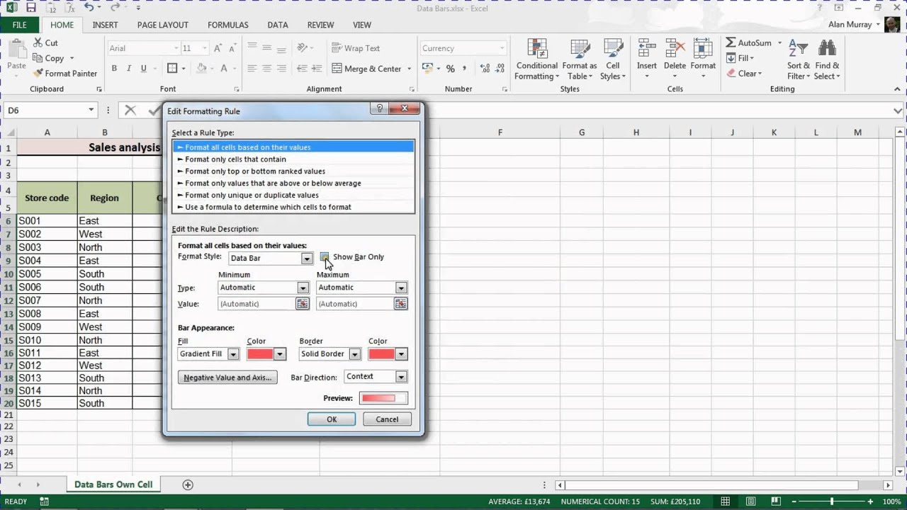
In the “Edit Formatting Rule” window, you will see the option to set the “Minimum” and “Maximum” values.
Click on the “Maximum” value field and enter the desired maximum value.
Click “OK” to apply the changes and close the window.

By manually adjusting the maximum value, you have control over the data bars’ visual representation. This allows you to emphasize the relative values of your data and create a more visually appealing representation in your Excel spreadsheet.

Using a Formula to Set the Maximum Value

Another way to define the maximum data bars value in Excel is by using a formula. This method allows you to dynamically set the maximum value based on the data range you are working with. Here’s how you can do it:

1. Select the cell where you want to set the maximum value for the data bars.

2. Enter the formula that will determine the maximum value. For example, if you want the maximum value to be the highest number in a range of cells, you can use the MAX function. The formula would look something like this: =MAX(A1:A10).

3. Press Enter to apply the formula. The cell will now display the maximum value based on the data range you specified.

4. Now, select the range of cells that you want to apply the data bars to.

5. With the range selected, go to the “Home” tab in the Excel ribbon and click on “Conditional Formatting” in the “Styles” group.

6. From the drop-down menu, select “Data Bars” and then click on “More Rules” at the bottom of the menu.

7. In the “Edit Formatting Rule” dialog box, select “Formula” from the “Type” drop-down menu.

8. Enter the formula that will compare each cell in the range to the maximum value cell. For example, if your maximum value cell is A1, you can use the formula: =$A1/A$1. This formula will calculate the percentage of each cell’s value relative to the maximum value.

9. Customize the appearance of the data bars as desired using the options in the “Edit Formatting Rule” dialog box.

10. Click “OK” to apply the data bars with the formula-based maximum value.

By using a formula to set the maximum value for the data bars, you can ensure that the bars accurately represent the range of values in your data and dynamically adjust as the data changes.

Using Conditional Formatting to Set the Maximum Value

If you want to automatically set the maximum value for your data bars in Excel, you can utilize the power of conditional formatting. This feature allows you to apply formatting rules based on specific criteria or conditions. By creating a conditional formatting rule, you can dynamically set the maximum value for your data bars. Here’s how:

1. Select the cells where you want to apply the data bars.

2. Go to the “Home” tab on the Excel ribbon and click on the “Conditional Formatting” button in the “Styles” group.

3. From the dropdown menu, choose “New Rule.”

4. In the “New Formatting Rule” dialog box, select “Format only cells that contain” under the “Select a Rule Type” section.

5. In the “Edit the Rule Description” section, select “Cell Value” from the first dropdown menu, “greater than or equal to” from the second dropdown menu, and enter the desired maximum value in the field.

6. Click on the “Format” button to specify the formatting for the cells that meet the condition.

7. In the “Format Cells” dialog box, go to the “Fill” tab and choose the desired fill color for the data bars.

8. Click “OK” to apply the formatting.

Now, the cells containing values equal to or greater than the maximum value you specified will be displayed with data bars. The length of the data bars will dynamically adjust based on the values in your selected range.

By using conditional formatting, you can easily set the maximum value for your data bars without the need to manually adjust them. This not only saves you time but also ensures that your data bars accurately represent the range of values in your dataset.

Creating a Custom Data Bar Format with Maximum Value

Excel allows you to create custom data bar formats to further enhance the visual representation of your data. By creating a custom data bar format, you can not only define the maximum value for the data bars but also add additional formatting options to make your data stand out.

To create a custom data bar format with a maximum value, you can follow these steps:

Select the range of cells containing your data. Make sure the cell containing the maximum value is included in the selection.
Click on the “Conditional Formatting” option in the “Home” tab of the Excel ribbon.
From the drop-down menu, select “Data Bars” and then click on “More Rules”.
A dialog box will appear. In the “Edit Formatting Rule” section, select the options that suit your needs, such as color, bar direction, and bar style.
Under the “Minimum” and “Maximum” sections, select the desired options to customize the data bar format according to your preference.
In the “Type” section, choose the option “Custom” to define the maximum value manually.
Enter the maximum value in the input box provided.
Click “OK” to apply the custom data bar format with the defined maximum value.

By creating a custom data bar format with the maximum value defined, you can visually represent your data in a way that is meaningful and impactful. This allows you to highlight the important aspects of your data and make it easier for others to interpret.

Remember, when creating a custom data bar format, you have the flexibility to choose different formatting options, including color, direction, and style. Experiment with different combinations to find the format that best suits your data and presents it in a visually appealing manner.

Creating a custom data bar format with a maximum value not only adds visual interest to your data but also enhances its comprehension. It allows you and your audience to quickly identify the significance of the data and make informed decisions based on it.

Conclusion

In conclusion, mastering the ability to define the maximum data bars value in Excel can significantly enhance your data visualization skills. By using this feature effectively, you can effortlessly make your data more understandable and visually appealing. Whether you want to highlight the highest value in a dataset or create meaningful data comparisons, the maximum data bars functionality can be a powerful tool in your data analysis arsenal.

By following the step-by-step instructions in this article, you can easily customize and control the maximum data bars value according to your specific data requirements. Remember to experiment with different settings and styles to find the best visual representation for your data.

Excel offers a wide range of data visualization features, and mastering these tools can empower you to present information in a more impactful way. So, take your data analysis skills to the next level by harnessing the power of Excel’s maximum data bars functionality!

FAQs

1. What is the maximum data bars value in Excel?
The maximum data bars value in Excel refers to the highest value that can be assigned to a data bar in a cell. It represents the maximum length that a data bar can visually display to represent a specific value in a range.

2. How do I define the maximum data bars value in Excel?
To define the maximum data bars value in Excel, you need to follow these steps:
a. Select the range of cells that you want to apply the data bars to.
b. On the Home tab, click on the Conditional Formatting button and choose Data Bars from the dropdown menu.
c. In the Data Bars submenu, select “More Rules” option.
d. In the Format Cells dialog box, specify the maximum value for the data bars by entering it in the “Maximum” field.
e. Click OK to apply the changes.

3. Why is it important to define the maximum data bars value in Excel?
Defining the maximum data bars value in Excel is important because it allows you to effectively represent data visually. By setting the maximum value, you can ensure that the length of the data bars accurately corresponds to the data values, providing a clear visual representation of the data range.

4. Can I change the maximum data bars value after applying them?
Yes, you can change the maximum data bars value after applying them in Excel. Simply repeat the steps mentioned in the previous question, and adjust the maximum value as per your requirements. The data bars will automatically adjust to reflect the new maximum value.

5. Are there any limitations to define the maximum data bars value in Excel?
Yes, there are limitations to define the maximum data bars value in Excel. The maximum value that you can assign to a data bar is limited by the length of the cell. If the data bar exceeds the cell size, it may not be fully visible or accurately represent the data. It’s important to consider the cell size and adjust the maximum value accordingly to ensure optimal visualization of the data bars.

How To Define Maximum Data Bars Value In Excel

Inside This Article