How To Group Data In Excel Pivot Table

Excel pivot tables are an incredibly powerful tool for analyzing and summarizing large amounts of data. They allow you to quickly and efficiently organize your data, perform calculations, and create insightful reports. One of the key features of pivot tables is the ability to group and categorize data based on specific criteria.

Grouping data in an Excel pivot table enables you to consolidate and summarize data by distinct categories, such as dates, months, or regions. This can be particularly useful when dealing with large datasets, as it allows you to focus on specific subsets of data and gain valuable insights.

In this article, we will explore how to efficiently group data in an Excel pivot table. Whether you are an Excel novice or a seasoned user, this guide will provide you with the necessary knowledge to leverage the power of pivot tables and make your data analysis more effective and efficient.

Inside This Article

1. Step 1: Create a Pivot Table in Excel
2. Step 2: Add Fields to the Pivot Table
3. Step 3: Group Data by Rows or Columns
4. Step 4: Customize Grouping Options
5. Conclusion
6. FAQs

Step 1: Create a Pivot Table in Excel

Creating a pivot table in Excel is a powerful way to analyze and summarize large amounts of data. With just a few simple steps, you can transform your raw data into organized and insightful reports.

To create a pivot table in Excel, follow these easy steps:

1. Open Excel and open the workbook that contains the data you want to analyze.
2. Select the data range you want to include in your pivot table. This can be a single column or a range of columns.
3. Go to the “Insert” tab in the Excel ribbon and click on the “PivotTable” button. This will open the “Create PivotTable” dialog box.
4. In the dialog box, make sure the “Select a table or range” option is selected. Verify that the correct range is displayed in the “Table/Range” box.
5. Choose where you want to place the pivot table. You can either place it on a new worksheet or on an existing worksheet.
6. Click “OK” to create the pivot table. Excel will generate the pivot table structure and display the PivotTable Field List.

Congratulations! You have successfully created a pivot table in Excel. Now it’s time to add fields and customize the table to meet your specific needs.

Step 2: Add Fields to the Pivot Table

After creating a Pivot Table in Excel, the next step is to add fields to it. Fields are used to determine how the data will be displayed in the Pivot Table. You can add different types of fields, such as data fields, column fields, and row fields.

To add a field, follow these steps:

1. Select the Pivot Table by clicking on any cell within the table.
2. Navigate to the “Field List” or “PivotTable Field List” (depending on your Excel version) on the right side of the Excel window.
3. Drag and drop the desired field to the appropriate section in the field list. For example, if you want to add a field to the columns, drag it to the “Columns” section. If you want to add it to the rows, drag it to the “Rows” section.
4. You can also select multiple fields to add by holding down the Ctrl key while selecting the fields.

Once you add the fields, Excel will automatically update the Pivot Table to display the data based on the selected field(s). You can add as many fields as you need to organize and analyze your data effectively.

Step 3: Group Data by Rows or Columns

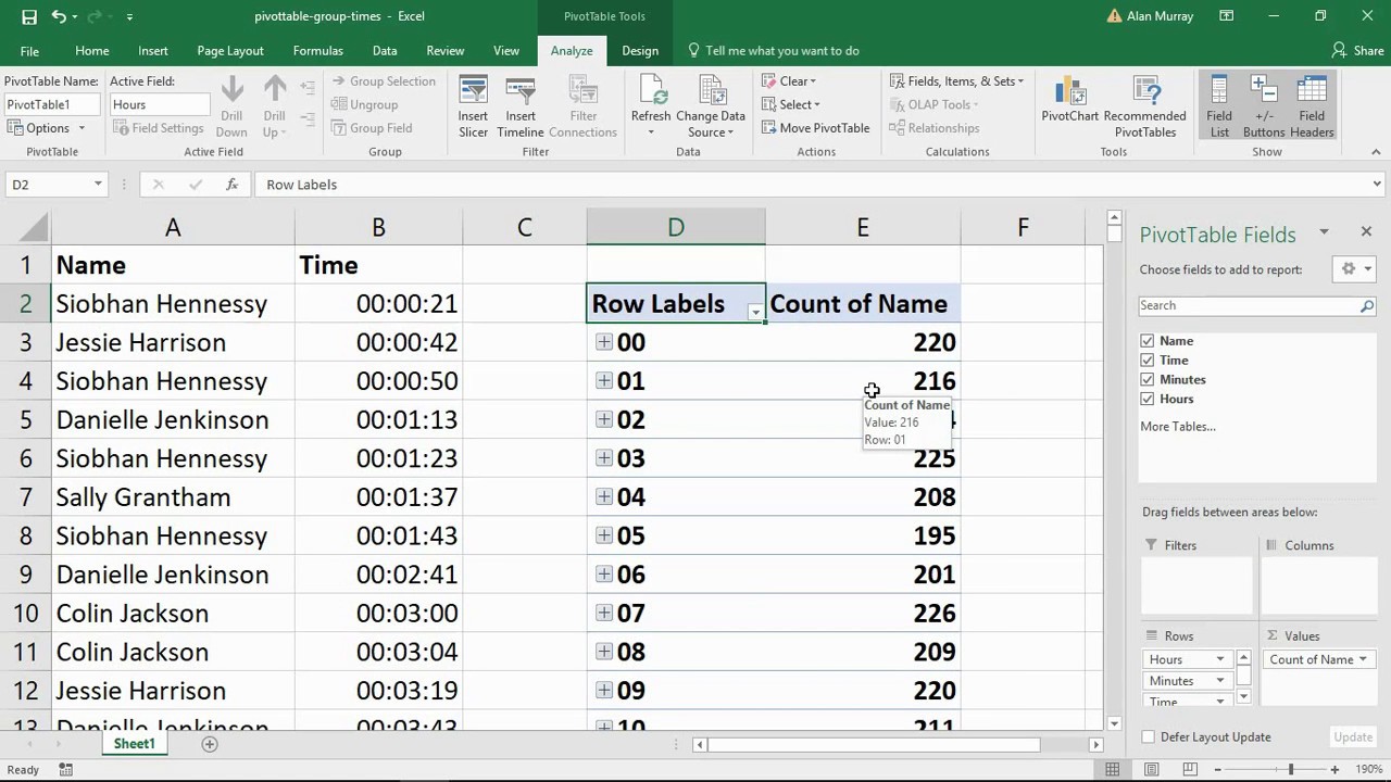
Once you have created a Pivot Table in Excel and added the necessary fields, it’s time to dive into grouping the data. Grouping data allows you to categorize and summarize your data based on specific criteria, making it easier to analyze and draw insights.

To begin, select the data in your Pivot Table that you want to group. This can be done by clicking on the cell within the Pivot Table and then selecting the “Group Selection” option under the “PivotTable Tools” tab.

Next, a dialog box will appear where you can choose how you want to group the data. You can either group by rows or columns, depending on your preference and the nature of your data.

If you choose to group by rows, you can select the specific field you want to group by. For example, if you have a Pivot Table with sales data for different regions, you can group the data by the “Region” field. This will then group all the data by region, making it easier to see the sales figures for each region.

Similarly, if you choose to group by columns, you can select the field you want to group by, such as the “Month” field if your Pivot Table contains monthly sales data. This will then group the data by month, allowing you to easily compare and analyze sales trends over time.

Once you have selected the field you want to group by and clicked “OK,” Excel will automatically group the data in your Pivot Table accordingly. You will now see the grouped data displayed in your Pivot Table, organized based on the criteria you specified.

It’s important to note that you can also customize the grouping options in Excel. For example, you can choose to group the data by a specific time period, such as grouping sales data by quarters or years. This can be done by right-clicking on the grouped data in your Pivot Table, selecting “Group” and then choosing the desired grouping interval.

Overall, grouping data in a Pivot Table is a powerful feature in Excel that allows you to organize and summarize your data more effectively. By grouping data by rows or columns, you can gain valuable insights and make better-informed decisions based on your analysis.

Step 4: Customize Grouping Options

Once you have grouped your data in a Pivot Table in Excel, you may want to further customize the grouping options to meet your specific needs. Excel provides several options to customize the way your data is grouped, allowing you to organize and analyze your data more effectively.

Here are some ways you can customize the grouping options in Excel Pivot Tables:

1. Change the grouping range: By default, Excel automatically determines the range for grouping based on the selected data. However, you can manually change the grouping range if needed. Simply right-click on a cell in the Pivot Table, select “PivotTable Options,” and go to the “Data” tab. Here, you can adjust the range under the “Data range” section.
2. Modify the grouping intervals: By default, Excel automatically determines the intervals for grouping based on the data values. However, you can modify these intervals to group the data in a different way. For example, if you are grouping a range of dates, you can change the grouping intervals from months to quarters or years. To do this, right-click on a grouped field in the Pivot Table, select “Group,” and adjust the intervals as desired.
3. Add additional grouping levels: If you want to further segment your data, you can add additional grouping levels to your Pivot Table. This is particularly useful when analyzing data with multiple dimensions. For example, if you have a Pivot Table with sales data categorized by region and month, you can add a third grouping level for product type. To add a grouping level, right-click on a grouped field in the Pivot Table, select “Group,” and choose the desired grouping option.
4. Customize the group labels: Excel allows you to customize the labels used for grouped data. This can be useful for displaying more meaningful and descriptive labels. To customize the group labels, right-click on a cell in the Pivot Table, select “PivotTable Options,” and go to the “Display” tab. Here, you can enter custom labels for each group.
5. Remove grouping: If you no longer need to group your data in a Pivot Table, you can easily remove the grouping. Simply right-click on a grouped field in the Pivot Table, select “Ungroup,” and the grouping will be removed.

By customizing the grouping options in Excel Pivot Tables, you can gain more control over how your data is organized and presented. This can help you to extract valuable insights and make informed decisions based on your data analysis. Experiment with different grouping options to find the configuration that best suits your needs.

In conclusion, mastering the skill of grouping data in an Excel pivot table opens up a world of possibilities for data analysis and reporting. The ability to group data by different criteria allows you to gain valuable insights, identify patterns, and extract meaningful information from large datasets efficiently.

By organizing information into logical groups, you can easily summarize and analyze data without the need for complex formulas or manual sorting. Grouping data in a pivot table helps you to visualize trends, make comparisons, and draw conclusions effectively.

With the step-by-step guide provided in this article, you can confidently navigate through the process of grouping data in your Excel pivot table. Whether you are analyzing sales data, financial records, or survey results, being able to group data will empower you to uncover valuable insights and make informed decisions.

So start experimenting with the group feature in your pivot table and unleash the full potential of your data analysis prowess!

FAQs

Q: What is a Pivot Table in Excel?

A: A Pivot Table in Excel is a powerful data analysis tool that allows you to summarize and analyze large amounts of data in a structured manner. It provides you with the capability to group and aggregate data based on different criteria, helping you gain valuable insights and make informed decisions.

Q: How do I create a Pivot Table in Excel?

A: To create a Pivot Table in Excel, follow these steps:

1. Select the data range that you want to analyze.
2. Go to the “Insert” tab in Excel’s menu bar.
3. Click on the “PivotTable” button and select “PivotTable” from the drop-down menu.
4. In the “Create PivotTable” dialog box, choose the location where you want the Pivot Table to be placed.
5. Drag and drop the fields from your data range into the “Rows”, “Columns”, and “Values” areas to define the structure of your Pivot Table.
6. Customize the Pivot Table settings, such as applying filters, sorting, and formatting, to suit your analysis needs.

Q: How can I group data in a Pivot Table?

A: To group data in a Pivot Table, follow these steps:

1. Select the data field that you want to group.
2. Right-click on the field and choose “Group” from the context menu.
3. In the “Grouping” dialog box, specify the range and interval for the grouping.
4. Click “OK” to apply the grouping to the Pivot Table.

Q: Can I group dates in a Pivot Table?

A: Yes, you can group dates in a Pivot Table. Excel provides various options for grouping dates in different intervals, such as by days, months, quarters, or years. This allows you to analyze your data based on specific time periods, making it easier to identify trends and patterns.

Q: Can I undo the grouping in a Pivot Table?

A: Yes, you can undo the grouping in a Pivot Table by following these steps:

1. Select the grouped field in the Pivot Table.
2. Right-click on the field and choose “Ungroup” from the context menu.
3. The grouped data will be reverted back to its original state.